Mid semester class test
CHEN4011 - Advanced Modelling and Control
Question 1 (10 marks)
Consider the following transfer functions for a mixing process:
G_P(s) = \frac{4 e^{-2s}}{3s+1}, \qquad G_D(s) = \frac{-6 e^{-s}}{(s+1)(2s+1)}
The system is controlled with a PI controller of the form
G_C(s) = K_c \left( 1 + \frac{1}{\tau_I s} \right),
with parameters K_c = 20, \, \tau_I = 4.
Assume unity measurement. The feedforward signal is added at the plant input. For parts (c)–(e), ignore the time delay.
Tasks:
- Derive the expression for the ideal feedforward controller G_{FF}(s). (2 marks)
Answer
The ideal feedforward controller is obtained from
G_{FF}^{\star}(s) = -\frac{G_D(s)}{G_P(s)}.
G_{FF}^{\star}(s) = -\frac{-6 e^{-s}/\big[(s+1)(2s+1)\big]}{4 e^{-2s}/(3s+1)} = \frac{3}{2}\,e^{+s}\,\frac{3s+1}{(s+1)(2s+1)}.
- Comment on whether it is realizable. If the ideal feedforward controller is not realizable, suggest practical strategies to approximate it. (2 marks)
Answer
The term e^{+s} corresponds to a time advance (prediction), which is non-causal and thus not physically realizable.
Practical approximations:
- Delay matching: Insert a deliberate 1 s delay to cancel the advance:
G_{FF}(s) = \frac{3}{2}\,\frac{3s+1}{(s+1)(2s+1)}\,e^{-s}. - Static gain feedforward: Use steady-state gain ratio with a filter:
G_{FF}(s) \approx -1.5\,\frac{1}{\tau_f s+1}. - IMC-style filtered inversion:
G_{FF}(s) = -\frac{G_D(s)}{G_P(s)}\,Q_{ff}(s), with Q_{ff}(s)=\big(1/(\tau_f s+1)\big)^n to enforce causality and robustness.
- Delay matching: Insert a deliberate 1 s delay to cancel the advance:
- Derive the open-loop transfer function G_{OL}(s). (2 marks)
Answer
Ignoring delays: G_P(s) = \frac{4}{3s+1}, \quad G_C(s) = 20\left(1+\frac{1}{4s}\right).
G_{OL}(s) = G_C(s) G_P(s) = \frac{20(4s+1)}{s(3s+1)}.
- Derive the closed-loop transfer function \tfrac{Y(s)}{Y_{sp}(s)} assuming unity feedback. (2 marks)
Answer
With unity feedback: \frac{Y(s)}{Y_{sp}(s)} = \frac{G_C(s)G_P(s)}{1+G_C(s)G_P(s)} = \frac{20(4s+1)}{s(3s+1)+20(4s+1)}.
Simplified: \frac{Y(s)}{Y_{sp}(s)} = \frac{80s+20}{3s^2+81s+20}.
- Using the Routh criterion, comment on the stability of the closed-loop system. (2 marks)
Answer
Characteristic polynomial: 3s^2 + 81s + 20.
- All coefficients are positive.
- For a second-order system, positivity of coefficients ensures stability.
- The discriminant 81^2 - 4\cdot 3 \cdot 20 = 6321 > 0, confirming real negative roots.
Conclusion: The closed-loop system is stable.
Question 2 (10 Marks)
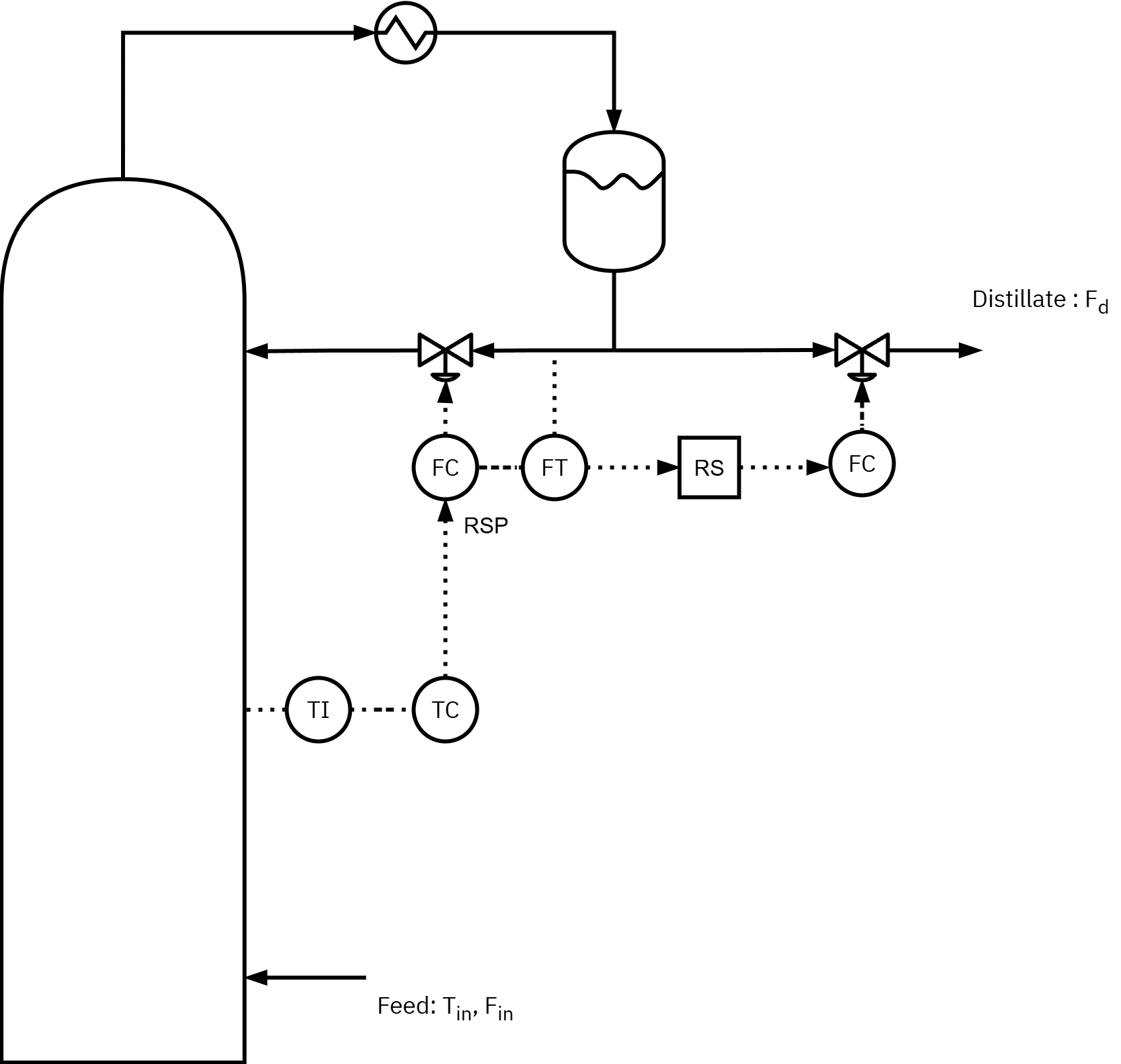
A binary distillation column has a total condenser and a reflux drum. The overhead vapor is condensed to liquid and split into reflux L back to the column and distillate D to product. The top‑tray temperature T_{tray} used as an inferential measure of distillate composition.
The plantwide policy is to hold a constant reflux‑to‑distillate ratio (R = L/D = 1.5) to stabilize top composition x_D during feed disturbances while the drum level is regulated. A ratio station computes the reflux‑flow setpoint from the measured distillate flow.
a). For ratio control identify the following (5 marks)
Controlled variable (CV) of the ratio loop:
Answer:
r = \dfrac{L}{D} held at set value R = 1.5
Measured variables used by the ratio station:
Answer
Distillate flow D_{\text{meas}} (optionally a trim signal from T_{tray} or x_D analyzer)
Manipulated variable (MV):
Answer
Reflux flow controller setpoint L_{\text{sp}} (reflux valve)
Ratio relationship implemented (write the exact formula the ratio station should use, including an optional trim b):
Answer
L_{\text{sp}} = R \, D_{\text{meas}} + b
Major disturbances the ratio loop helps reject (list any three):
Answer
Major disturbances the ratio loop helps reject (any three):
- Feed flow-rate changes
- Feed composition changes
- Feed temperature/enthalpy changes
- Upstream pressure fluctuations
- Condenser cooling-water temperature changes
Regulatory control for safe operation (name the variables typically held and their actuators):
Answer
Regulatory control for safe operation (variables and actuators):
- Reflux drum level → distillate product valve
- Column pressure → condenser duty or vent/blanket valve
- Reboiler (sump) level → bottoms product valve
- Reboiler heat input → steam or heat-medium valve
- Feed flow → feed control valve
b). Draw a clean schematic showing a cascade control structure in which the tray‑temperature controller is the primary loop and a reflux‑to‑distillate ratio controller is the secondary loop feeding the reflux flow controller. (5 marks)
Question 3 (10 Marks)
Consider the process
G_p(s)=\frac{5\,e^{-3s}}{(4s+1)(s+1)}.
A PI controller is used with parameters
K_c=0.2,\qquad \tau_I=4.
Develop a SIMULINK model to simulate:
- Standard feedback control with PI only.
- Smith Predictor based control. Use the internal model without delay,
G_m(s)=\frac{5}{(4s+1)(s+1)},
and place the actual time delay only in the forward plant path.
Use the following conditions while developing the simulation.
- Total simulation time: 100 s
- Set point: unit step at t=0
- Use the PI parameters above for both cases
- Measure output y(t)
Upload the developed SIMULINK model to the submission link on blackboard.
Populate Table 1.
| Performance metric | PI only | Smith Predictor |
|---|---|---|
| Settling time | ||
| (within 2% of nominal value) | 44.6 | 14.7 |
| Overshoot | 44.43 % | 0 |
| Undershoot | 19.16% | 0 |
| ISE | 6.286 | 2.5 |
Question 4 (10 Marks)
A DC motor is driven by an input voltage and both the angular position and angular velocity are measured as outputs. The dataset dcmotordata is provided with MATLAB System Identification Toolbox. It contains:
u: armature voltage (input)y: [angular position, angular velocity] (outputs)
Load the data in MATLAB with the commands:
load dcmotordata
z = iddata(y,u,0.1);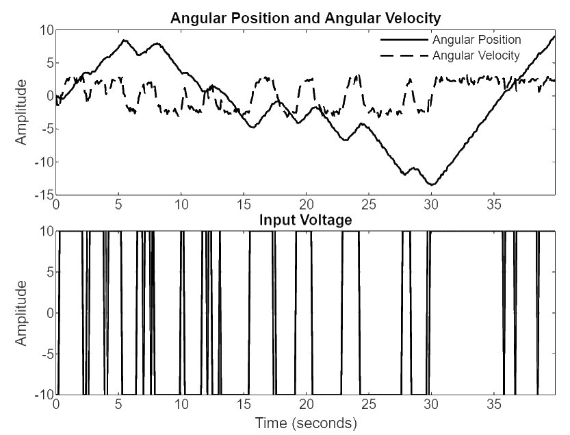
Here, y includes two outputs and 0.1 is the sampling time (s).
Use the first 200 samples of the dataset (z(1:200)) for model estimation and the last 200 samples (z(201:400)) for model prediction (testing).
Estimate the following multi-output models using MATLAB functions:
- Transfer function models with one and two poles (
tfest) - ARX models with orders (na=2, nb=2, nk=1) and (na=4, nb=4, nk=1) (
arx) - ARMAX model with orders (na=2, nb=2, nc=2, nk=1) (
armax)
- Compare each model against the test data using the
comparecommand. Report the fit percentage for prediction data in Table 2 for both outputs. (5 marks)
| Model | Fit to angular position data | Fit to angular velocity data |
|---|---|---|
| Transfer function with one pole | ||
| Transfer function with two poles | ||
| ARX model (na=2, nb=2, nk=1) | ||
| ARX model (na=4, nb=4, nk=1) | ||
| ARMAX model (na=2, nb=2, nc=2, nk=1) | ||
Answer
| Model | Fit to angular position data | Fit to angular velocity data |
|---|---|---|
| Transfer function with one pole | 91.22 | 84.47 |
| Transfer function with two poles | 98.35 | 84.49 |
| ARX model (na=2, nb=2, nk=1) | 97.37 | 83.44 |
| ARX model (na=4, nb=4, nk=1) | 97.78 | 84.38 |
| ARMAX model (na=2, nb=2, nc=2, nk=1) | 98.26 | 84.82 |
- Comment on the results. (5 marks)
- Which output is harder to model?
Answer
The angular velocity output is consistently more difficult to model. Across all models, its fit percentage remains lower (≈83–85%) compared to the angular position output (≈91–98%). This suggests that the angular velocity exhibits more noise or faster dynamics that are not fully captured by the identified models.
- Does increasing model complexity always improve prediction? Explain why or why not.
No, increasing complexity does not guarantee better prediction.
For angular position, moving from a one-pole transfer function to a two-pole or higher-order ARX/ARMAX improves the fit significantly.
For angular velocity, however, increasing the order of ARX or moving to ARMAX yields only marginal improvements (less than 1%).
More complex models risk overfitting the estimation data, capturing noise rather than system dynamics, which does not translate into better performance on unseen test data.
Conclusion: A moderate-complexity model such as the ARMAX (2,2,2,1) provides a good balance—achieving excellent accuracy for angular position and the best (though still limited) accuracy for angular velocity without unnecessary over-parameterization.
Formula sheet
Ideal PI Controller Tuning
G_c = K_c \left( 1 + \frac{1}{\tau_I s} \right)
K_c = \frac{1}{K_P \tau_{ratio}}. Typically 1 < \tau_{ratio} < 5; \tau_I = \tau_P. Matlab controller parameters: P = K_c ; I = 1/\tau_I.
First-Order plus Deadtime (FOPDT) model
G(s) = \frac{K_p e^{-\theta s}}{\tau_p s + 1}
Idealized Feedforward Controller
G_{FF} = - \frac{G_D}{G_P}
Simple feedback loop with output disturbance
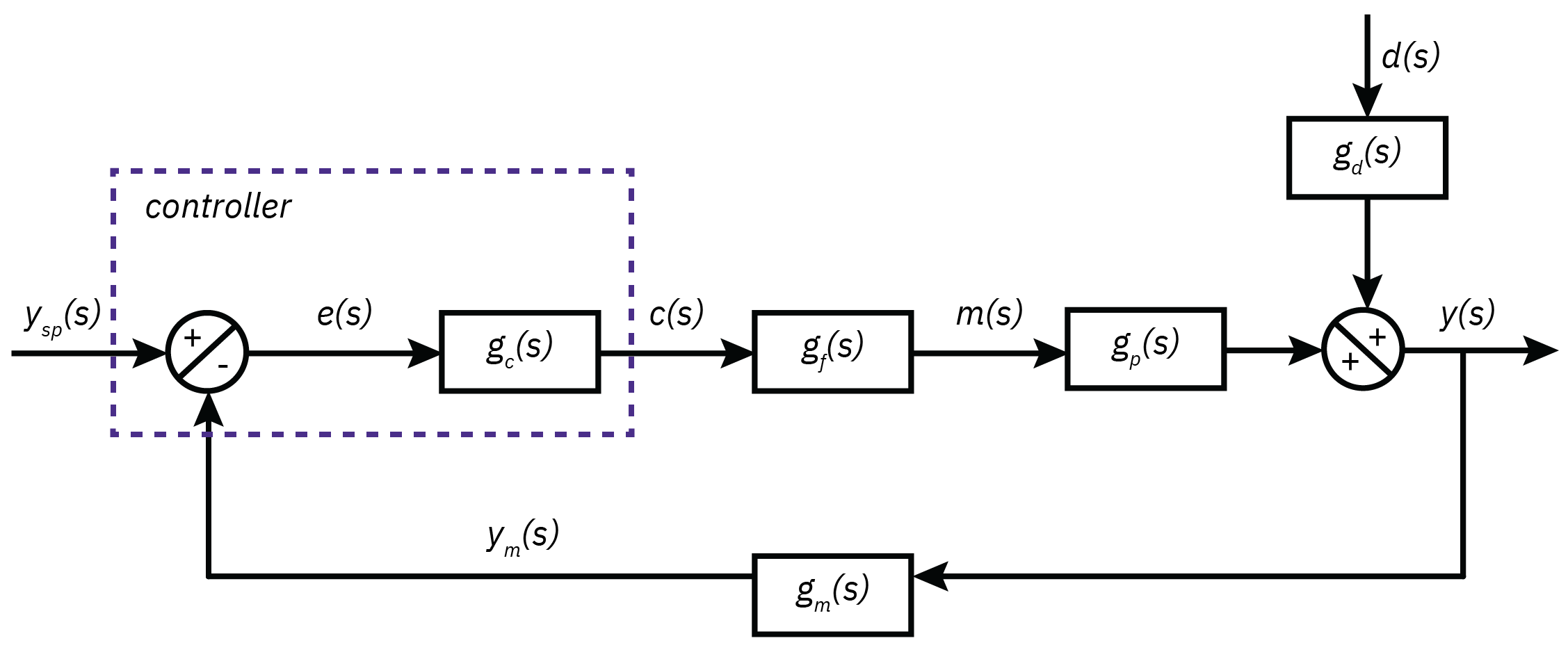
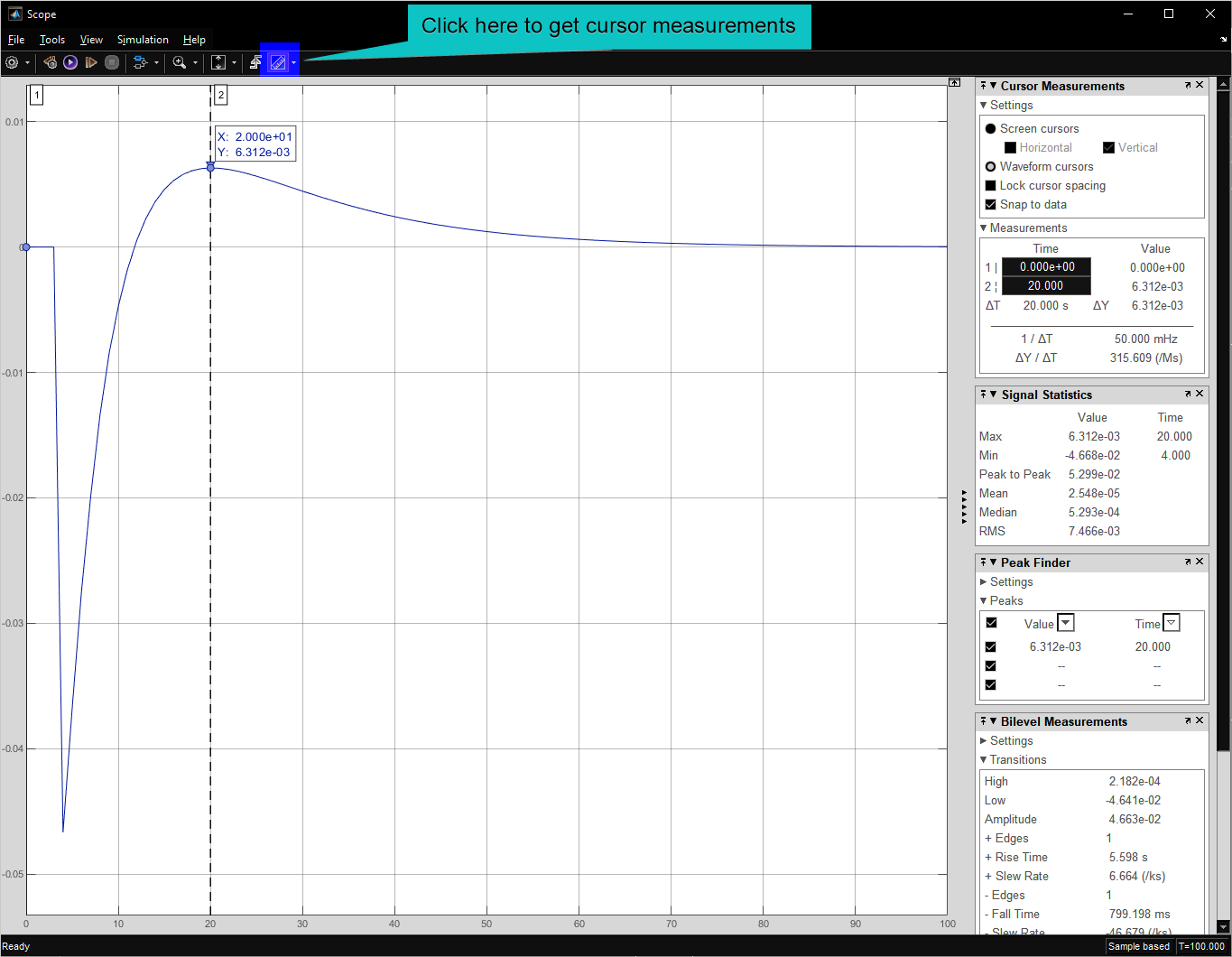
Cursor measurements
Useful information about the time series can be obtained using cursor measurements.
Citation
@online{student_id:,
  author = {Student ID:, Name:\textbackslash hspace\{8cm\}},
  title = {Mid Semester Class Test},
  url = {https://amc.smilelab.dev/admin/midsem/},
  langid = {en}
}