Basics of Process Control and Modeling

Lecture notes for Advanced modeling and Control

Lecture resources

Importance of process analysis and control

Chemical processes greatly influence every aspect of our life. All important industrial sector such as food production, water treatment, healthcare and pharmaceuticals, energy, automotives, and so on rely on chemical process industry to supply ingradients, raw materials, and enabling technologies. In recent years, significant attention is given to sustainability in the chemical process industry. New processes and retrofit of existing processes are based on responsible resource utilization, minimization of environmental impact, and considerations to long-term viability and competitiveness. Chemical processes involve several unit operations, such as mixing, heat exchange, mass transfer, and reaction. In a chemical process, required unit operations are performed in a specific sequence to achieve specific objectives. In order to ensure optimal operations of the process it is important to have efficient and effective control over process variables such as temperature, pressure, flow rate, and composition. Optimal operations are crucial for maintaining safety, and achieving desired product quality. Control systems and advanced algorithms are deployed to monitor, regulate, and optimize the process variables.

Controlling processes involves influencing their operation to achieve desired outcomes. This is accomplished through the use of control units, which regulate and guide processes to maintain steady operation and prevent deviations from target conditions. It is important to recognize that all industrial processes are dynamic, meaning their behavior changes over time. Control engineers must have a deep understanding of process dynamics and develop suitable mechanisms to influence and manage their behavior effectively.

Control engineering is an integral part of chemical engineering. Design engineers must account for dynamic operation and its consequences, while plant operators must respond to disruptions for smooth operation. Experimental engineers rely on process control for precise conditions. Without process control, modern processing facilities cannot operate safely, reliably, and profitably while meeting quality and environmental standards.

Process control objectives

Process System, Input and Output A process system refers to a collection of

interconnected components and equipment that work together to transform inputs into desired outputs in industrial or chemical processes.

Several key terms define the components of a control system, including Manipulated Variables (MV), Controlled Variables (CV), disturbances, and unmeasured outputs.

Figure 1: Process system nomenclature

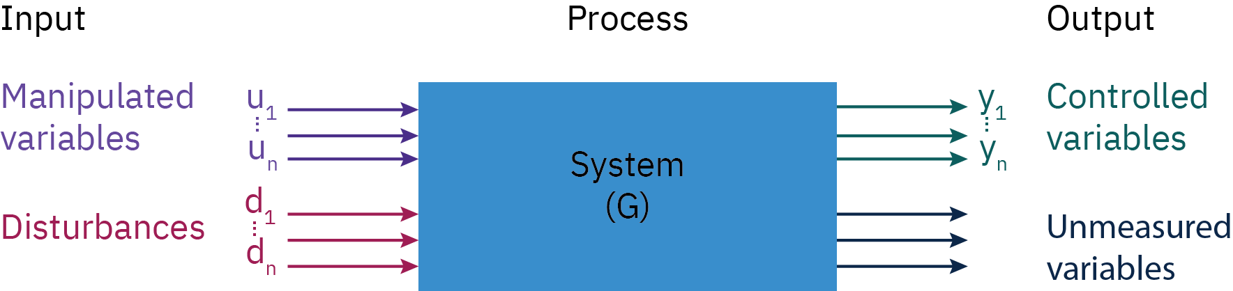
1. Manipulated Variables (MV): These are the inputs that a control system can adjust to influence the process. For example, in a heating system, the fuel supply to the burner could be a manipulated variable; the control system can increase or decrease the fuel supply to control the system.

2. Controlled Variables (CV): These are the outputs of the process that the control system aims to regulate. The control system adjusts the MVs to keep the CVs at their desired levels, known as setpoints. In the heating system example, the temperature of the room would be the controlled variable.

3. Disturbances: These are factors that can influence the CV but are not controllable by the system. They can be measurable or unmeasurable. In the heating system example, a disturbance could be the outside temperature. If it’s cold outside, it might cause the room temperature (CV) to decrease, so the control system needs to adjust the fuel supply (MV) to maintain the desired room temperature.

4. Unmeasured Outputs: These are the outputs of the process that are not directly controlled or measured, but may still be of interest. These could include quantities like efficiency, product quality, or environmental emissions. Because they are not directly measured, their values may need to be inferred from other variables or estimated using a process model.

Let’s consider a tank that’s used to store a liquid. The objective is to maintain the level of the liquid in the tank at a desired value. For this system MV, CV, disturbances, and unmeasured output can be identified as below.

Figure 2: liquid level in a tank

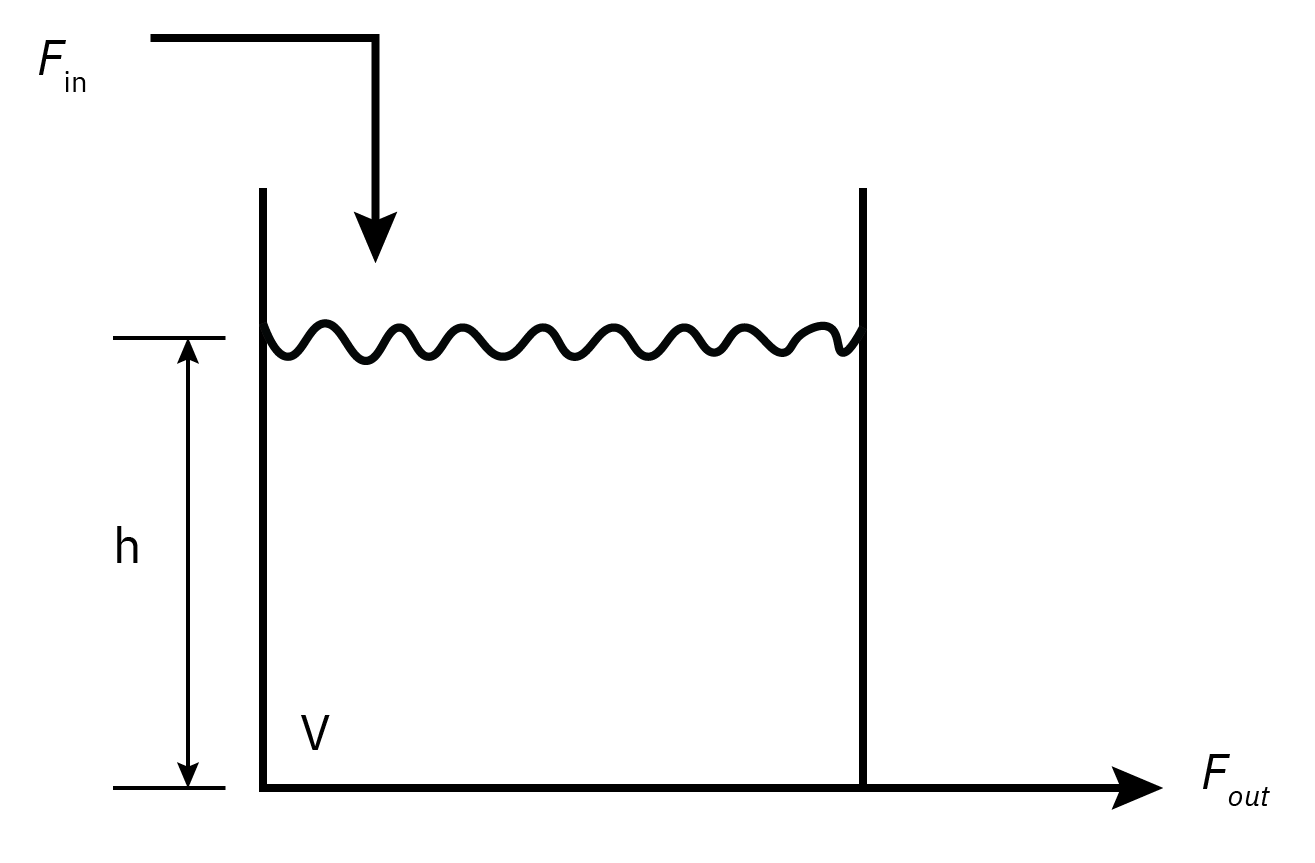
1. Manipulated Variable (MV): The flow rate of the liquid into or out of the tank. By increasing or decreasing the flow rate, the control system can regulate the level of the liquid.

2. Controlled Variable (CV): The level of the liquid in the tank. The control system measures the level and compares it to the setpoint, and then adjusts the manipulated variable (flow rate).

3. Disturbances: Changes in inlet flow rate, changes in outlet flow rate, temperature variations, pressure fluctuations, or any other factors that can impact the liquid level.

4. Unmeasured Output: An example of an unmeasured output could be the temperature of the liquid in the tank. While the control system may not directly measure the temperature, changes in temperature can affect the liquid’s density and, in turn, impact the level control dynamics. The control system must consider such unmeasured outputs and adjust the control strategy accordingly.

Implicit and explicit control objectives Both implicit and explicit control

objectives refer to the desired outcomes or goals for a system’s performance. They provide the framework for designing and tuning control systems.

Explicit Control Objectives

Explicit control objectives are clearly defined and typically quantifiable goals for the performance of a control system. These objectives are explicitly stated and usually include desired system responses such as stability, speed of response, minimal overshoot, accuracy, and robustness to disturbances. They may also include compliance with safety and environmental regulations. Explicit control objectives form the basis of the formal design and analysis of control systems (Seborg et al. 2016).

Some examples of explicit objectives are given below:

1. Setpoint Tracking: The control system should be able to maintain a process variable (such as temperature, pressure, or flow rate) at a desired setpoint. For example, a temperature control system in a reactor might have an explicit objective to maintain the temperature at 175°C.

2. Disturbance Rejection: The control system should be able to minimize the impact of disturbances on the process variable. For example, if a disturbance causes the temperature in a reactor to increase, the control system should bring it back to the setpoint as quickly and smoothly as possible.

3. Stability: The control system should maintain stability in the face of disturbances or setpoint changes. This means that it should not induce oscillations or lead to runaway conditions.

4. Speed of Response: The control system should achieve its control objectives quickly. This involves minimizing the rise time (the time it takes for the process to go from 10% to 90% of the final value) and settling time (the time it takes for the process to settle within a certain percentage of the final value).

5. Overshoot Minimization: When a setpoint change or disturbance occurs, the system should minimize overshoot, which is the extent to which the process variable exceeds the final value.

6. Regulatory Compliance: The control system should ensure that the process meets any applicable regulatory requirements. For instance, a control system for an industrial waste treatment process might have an explicit objective to maintain pollutant concentrations below regulatory limits.

Implicit Control Objectives

Implicit control objectives are usually not explicitly stated or quantified, but are understood to be desirable or necessary. Implicit objectives are often evaluated qualitatively, and they can have a significant impact on the long-term success of a control system. While explicit control objectives usually take precedence, implicit control objectives play a crucial role in the successful implementation and operation of control systems (luyben1990?).

Examples of implicit control objectives include:

1. Simplicity: The control system should be as simple as possible, making it easy to understand, implement, and maintain. For instance, a PID controller might be preferred over a more complex control strategy for a relatively simple process.

2. Reliability: The control system should operate reliably under normal and abnormal conditions. This could involve factors like hardware reliability, software robustness, and fault tolerance.

3. Cost-effectiveness: The cost of implementing and maintaining the control system should be reasonable. This includes not only the cost of hardware and software but also the cost of any downtime caused by control system issues.

4. Safety: While safety is often an explicit objective, it can also be an implicit goal in the sense that all control systems should inherently contribute to safe operation. This includes avoiding dangerous conditions and responding appropriately to emergency situations.

5. Flexibility: The control system should be adaptable to changes in the process or operating conditions. This could include the ability to handle different operating modes or the ability to be easily updated or reconfigured.

6. Scalability: The control system should be capable of handling increases in process size or complexity without a significant degradation in performance.

Implicit control objectives of process control

Control systems play a crucial role in ensuring safe and profitable operation of processes involving various streams. These control systems continuously monitor process variables such as temperature, pressure, level, flow, and concentration. They take actions, such as adjusting valves, controlling pump speed, and regulating heaters, to maintain these variables at specified set point values defined by operators. This enables processes to operate efficiently, meeting desired objectives while prioritizing safety and profitability.

The primary objective of any control system is safety. Control systems are designed to ensure the safety of people, protect the environment, and safeguard equipment. By continuously monitoring and adjusting process variables, these systems can detect and respond to deviations or disturbances that may pose risks or compromise the integrity of the system. This proactive approach to safety helps prevent accidents, minimize environmental impact, and preserve the longevity of equipment.

When faced with competing objectives, the specific tradeoff considerations vary depending on the industry, scale, and potential consequences involved. For example, In extreme scenarios such as a nuclear plant, the control system may shut down the operations to prevent potential deadly radiation leaks. On the other hand, in power or chemical industry, there is a tradeoff between controlling emissions and equipment safety. In order to keep the operations running optimally, the control system may deviate from the emission norms occasionally. Stricter emission control measures, may place additional stress on equipment and require diligent maintenance to ensure safe operation. Balancing emissions control with equipment safety becomes crucial to mitigate environmental harm while ensuring the integrity and reliability of the industrial process.

In addition to safety, automatic control also enhances efficiency and performance. By maintaining process variables at optimal set points, these systems enable processes to operate at peak efficiency, reduce energy consumption, improve product quality, and increase overall productivity. This not only maximizes output and profitability but also contributes to sustainability efforts by minimizing resource wastage and emissions.

After ensuring the people, environment, and equipment safety objectives are met, the control objectives can focus on the profit.

Plant-level control objectives motivated by profit include:

• meeting final product specifications
• minimizing waste production minimizing environmental impact minimizing energy use maximizing overall production rate

::: {#fig-process-variability layout=“[48,-4,48]”}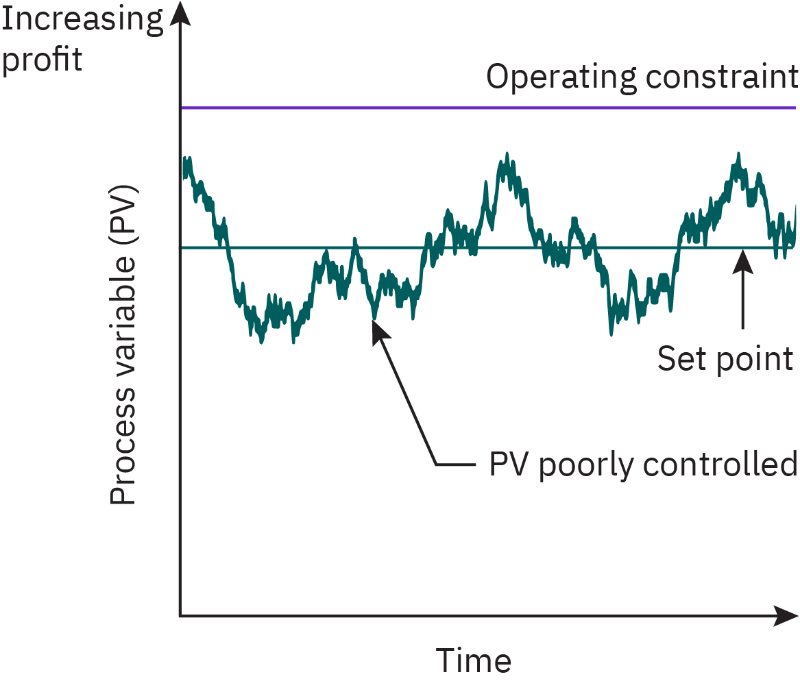

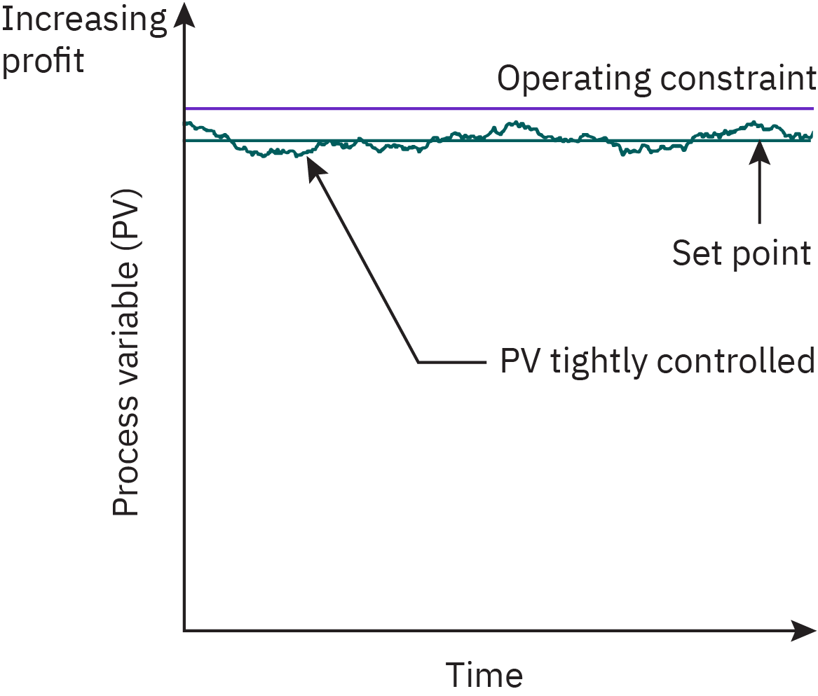
Figure 3: Good control permits set point near constraint

Process control plays a vital role in reducing variability :::

Control and Optimization

Both control and optimization share the common goal of improving the performance of a system, but they focus on different aspects and are used in different contexts.

Control involves adjusting an input variable to maintain an output variable at a desired value. This is accomplished using a control strategy, which continually measures the output, compares it with the desired value, and adjusts the input to minimize the difference or error between the desired value and output. Control is a dynamic process that occurs in real time. It’s primarily concerned with maintaining stability, reducing variability, and reacting to disturbances in the system.

On the other hand, optimization involves finding the best possible value of an output or set of outputs. In the context of process control, optimization often involves determining the best setpoint that will maximize or minimize a certain objective function (such as profit, energy usage, or waste production).

Optimization is often a higher-level task that takes place over a longer timeframe. The optimization of process operating conditions aims to maximize economic objectives, such as annual profit. Effective plant management involves determining desirable operating targets and implementing an efficient automatic control strategy to maintain these targets within acceptable limits. Chemical engineers are well-suited for setting control objectives as they possess a clear understanding of how the plant operates.

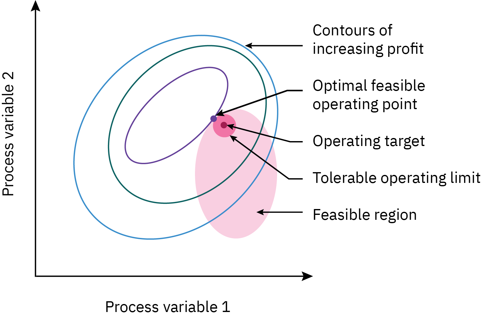
To identify the most desirable operating conditions, the feasible region of operation is defined based on the physical limits of decision variables. Plant economics are then evaluated by assessing increasing profit contours. While the optimum operating point often lies at a corner of the feasible region, practical considerations and plant disturbances necessitate operating at a slight distance from this point to ensure feasible operation (Figure 4).

The control strategy focuses on minimizing variations around the operating target and reducing the acceptable operating limits. Advanced control systems offer the potential for operating even closer to the optimal target, resulting in increased profitability. This improvement, quantified by a shift towards a more profitable regime, demonstrates the financial benefits of the control system.

Figure 4: Optimal plant operations

Hirarchy of process control activities

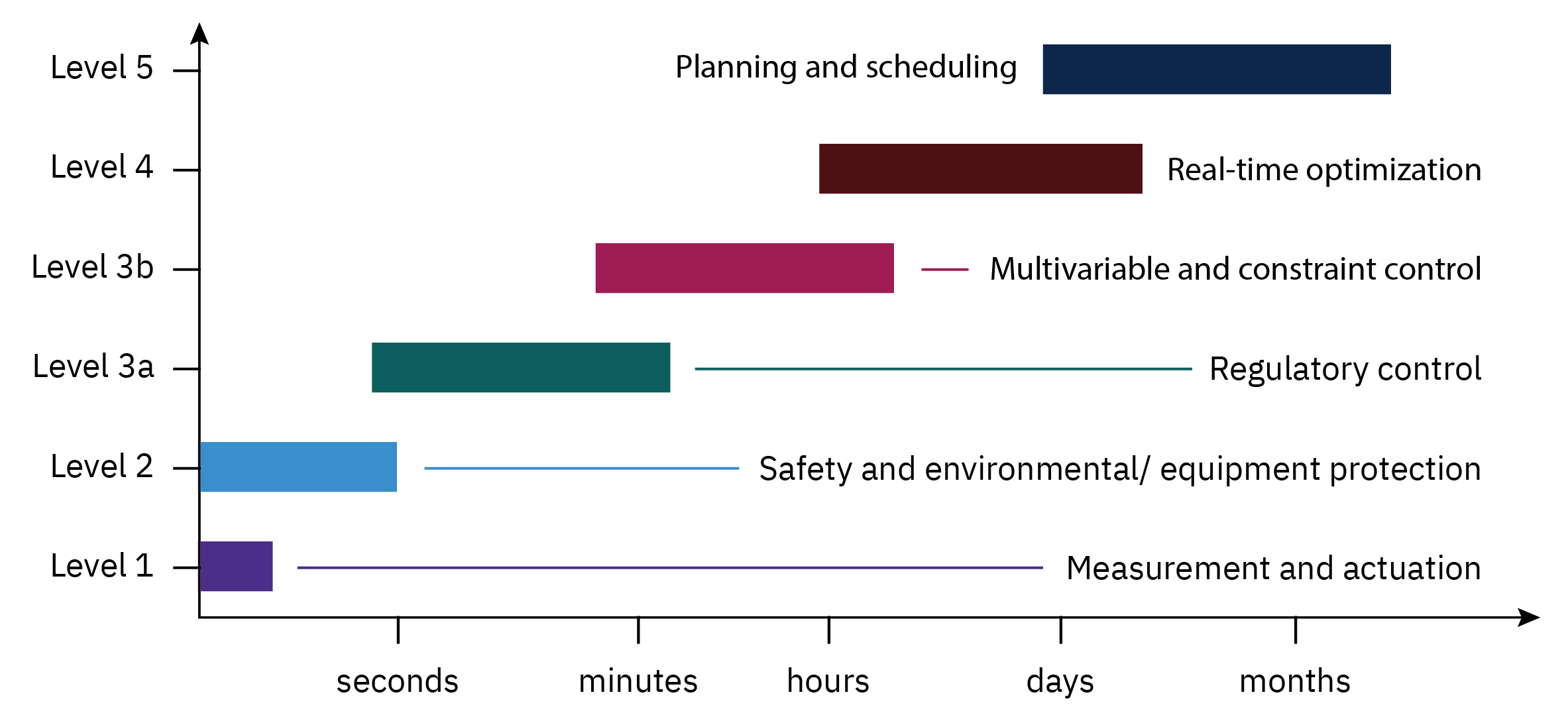
The hierarchy of process control activities is shown in Figure 5.

Measurement and Actuation (Level 1)

Instrumentation, which includes sensors and transmitters, is used to measure variables in a process. Actuation equipment, such as control valves, is employed to carry out the control actions determined by these measurements. In essence, measurement and actuation functions are fundamental components of any control system, as they enable the system to gather data about the process and respond accordingly to maintain optimal conditions or meet set parameters.

Safety and environmental/ equipment protection (Level 2)

Level 2 functions are essential in ensuring both the safety of the process and its compliance with environmental regulations. As discussed in Chapter 10, the approach to process safety involves the establishment of multiple layers of protection, consisting of various equipment and human actions.

A layer of this protection includes process control functions, like managing alarms during unusual situations and utilizing safety instrumented systems for emergency shutdowns. The safety gear, which encompasses sensors and control valves, functions independently of the standard instrumentation used for regulatory control in Level 3a.

Methods for validating sensor functionality can be utilized to verify that these sensors are operating correctly.

Regulatory control (Level 3a)

The successful operation of a process requires that critical process variables, such as flow rates, temperatures, pressures, and compositions, are managed at or near their specified set points. This activity, known as regulatory control, is achieved by applying standard feedback and feedforward control techniques.

However, if these conventional control methods are not sufficient, a range of advanced control techniques is at our disposal. In recent times, there’s been an increasing interest in the performance monitoring of control systems.

Multivariable and constraint control (Level 3b)

Many challenging process control issues have two key characteristics: they involve significant interactions among important process variables and they have inequality constraints for manipulated and controlled variables. These constraints, which include upper and lower limits, could be based on the capabilities of equipment or operational objectives for the process.

Operating a process near a constraint limit is a significant goal for advanced process control. In many industrial operations, optimal conditions are often at the constraint limit. However, the set point should not be the constraint value to prevent surpassing the limit due to disturbances. Therefore, it’s critical to set a conservative set point depending on the control system’s capacity to minimize disturbances.

Standard process control techniques might not be sufficient for managing complex control problems that involve severe process interactions and inequality constraints. In such cases, advanced control methods should be considered, including multivariable control and constraint control. Specifically, the model predictive control (MPC) strategy is designed to handle process interactions and inequality constraints.

Real time optimization (Level 4)

The optimal operating conditions for a plant are established during the process design phase. However, during the operation of the plant, these conditions can frequently change due to variations in equipment availability, process disturbances, and economic circumstances such as changes in raw material costs and product prices. As a result, it can be highly beneficial to frequently recalculate the optimal operating conditions. This activity, known as real-time optimization (RTO), involves implementing new optimal conditions as set points for controlled variables.

The RTO calculations are based on a steady-state model of the plant and economic data like costs and product values. The usual objective of the optimization is to either minimize operating costs or maximize operating profits. RTO calculations can be conducted for an individual process unit or for the whole plant.

Level 4 activities also incorporate data analysis to confirm the accuracy of the process model used in the RTO calculations under current conditions. Therefore, data reconciliation techniques can be utilized to ensure that steady-state mass and energy balances are met. Additionally, the process model can be updated using parameter estimation techniques and recent plant data.

Planning and scheduling (Level 5)

The highest tier of the process control hierarchy is focused on strategizing and orchestrating operations for the entire plant. For continuous processes, the production rates of all products and intermediates need to be planned and harmonized. This involves considering equipment limitations, storage capacity, sales forecasts, and the operations of other plants, which can sometimes be globally distributed.

For the intermittent operation of batch and semi-batch processes, production control transforms into a batch scheduling issue, guided by similar considerations. Hence, planning and scheduling tasks present challenging optimization problems that are founded on both engineering factors and business forecasts.

Figure 5: Hirarchy of process control activities

Overview of control system design

Control System Design of a plant involves two parts, namely, control structure design, and controller algorithm design.

Control Structure Design

The first step in designing a control system for a plant is defining the control structure. This includes deciding which variables to control (Controlled Variables, CVs), which variables to adjust (Manipulated Variables, MVs), and the structure that links these two sets of variables.

1. Controlled Variables (CVs): These are the variables that the control system aims to maintain at a certain level or setpoint. In a chemical reactor, for instance, you might want to control the temperature, pressure, or concentration of a certain species. The selection of CVs depends on the objectives of the process, such as product quality, safety, or environmental compliance.

2. Manipulated Variables (MVs): These are the variables that the control system can adjust to influence the CVs. In a reactor, these could include the flow rate of the reactants, the cooling rate, or the stirring speed. The selection of MVs depends on their influence on the CVs and their controllability.

3. Structure Linking CVs and MVs: Once the CVs and MVs are selected, the next step is to decide how they should be linked. In a single-loop control system, each CV is paired with one MV. In more complex systems, you might use multivariable control strategies where each MV can influence multiple CVs and vice versa. The structure should be designed to achieve the best control performance while considering practical aspects such as equipment limitations and interaction between variables.

Controller Algorithm Design

Once the control structure is defined, the next step is to design the control algorithm. This involves selecting the type of controller and tuning its parameters.

1. Controller Type: This could be a simple PID (Proportional-Integral-Derivative) controller, which is widely used in the industry due to its simplicity and effectiveness. For more complex systems, advanced control strategies like Model Predictive Control (MPC) might be used. The selection of controller type depends on the complexity of the process, the required performance, and the available resources.

2. Controller Tuning: This involves adjusting the parameters of the controller to achieve the best control performance. For a PID controller, this includes the proportional, integral, and derivative gains. For an MPC controller, this might involve tuning the prediction and control horizons, weights in the cost function, and model parameters.

Model based control

Model-based control represents a significant advancement in control engineering and has become increasingly important due to the growing complexity of systems and the need for improved performance. In model-based control, a mathematical model of the process is used to predict future outputs and decide on control actions. This approach allows for optimal control decisions, the handling of constraints, and the accommodation of system nonlinearity and multivariable interactions.

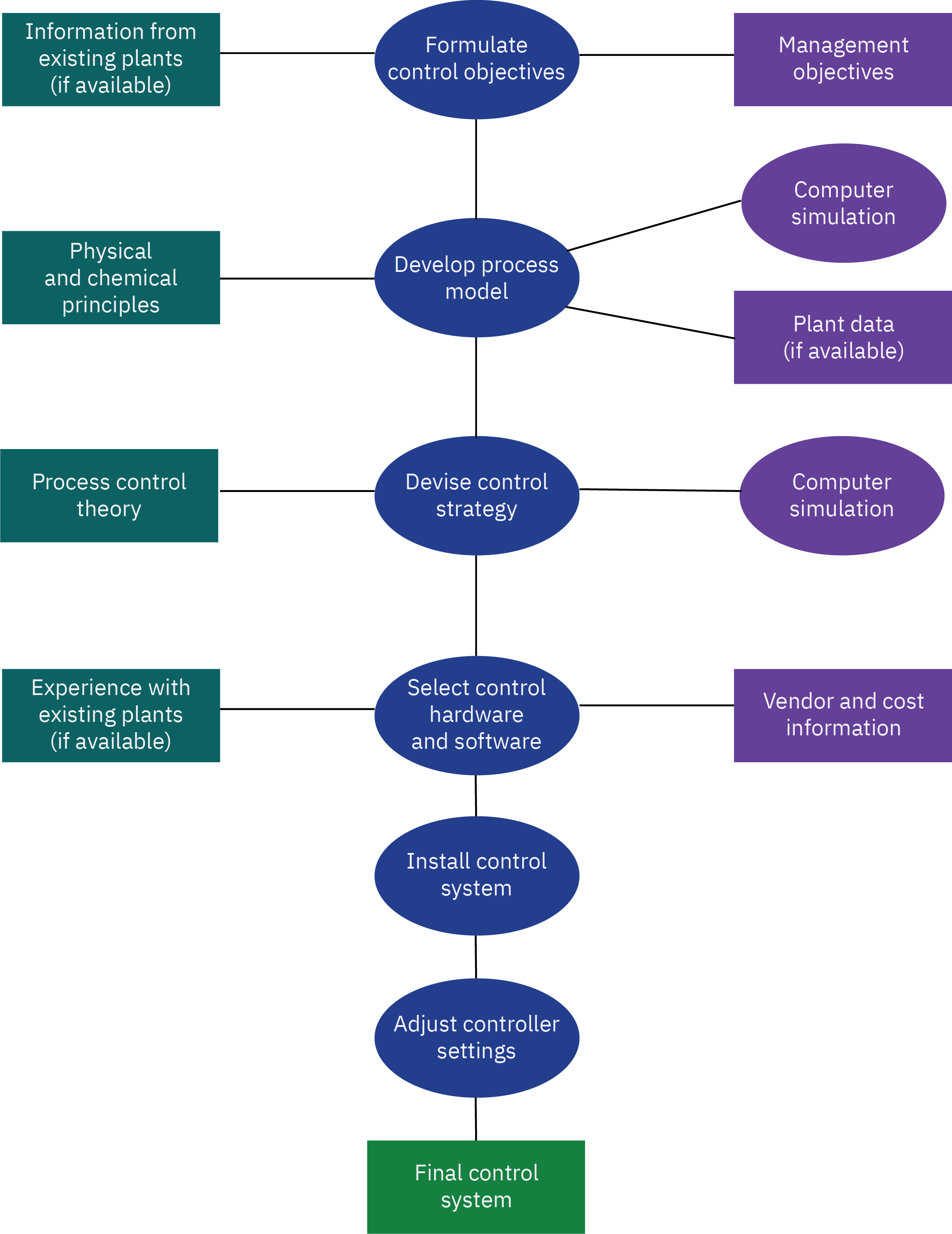
The major steps involved in designing and installing a control system using the model-based approach are shown in the flow chart of Figure 6. The first step, formulation of the control objectives, is a critical decision. The formulation is based on the operating objectives for the plants and the process constraints. For example, in the distillation column control problem, the objective might be to regulate a key component in the distillate stream, the bottoms stream, or key components in both streams. An alternative would be to minimize energy consumption (e.g., reboiler heat duty) while meeting product quality specifications on one or both product streams. The inequality constraints should include upper and lower limits on manipulated variables, conditions that lead to flooding or weeping in the column, and product impurity levels. After the control objectives have been formulated, a dynamic model of the process is developed. The dynamic model can have a theoretical basis, for example, physical and chemical principles such as conservation laws and rates of reactions, or the model can be developed empirically from experimental data. If experimental data are available, the dynamic model should be validated, and the model accuracy is characterized. This latter information is useful for control system design and tuning. The next step in the control system design is to devise an appropriate control strategy that will meet the control objectives while satisfying process constraints. As indicated in Figure 6, this design activity is both an art and a science. Process understanding and the experience and preferences of the design team are key factors. Computer simulation of the controlled process is used to screen alternative control strategies and to provide preliminary estimates of appropriate controller settings. Finally, the control system hardware and instrumentation are selected, ordered, and installed in the plant. Then the control system is tuned in the plant using the preliminary estimates from the design step as a starting point. Controller tuning usually involves trial-and-error procedures.

Figure 6: Major steps in control system development.

Introduction to process modeling

Dynamic models are crucial in the field of process dynamics and control.

• They enhance process understanding by allowing the study of transient behavior without disrupting the actual process. Through computer simulations, we can gain valuable insights into both dynamic and steady-state process behaviors, providing useful information even before a plant is constructed.

• Process simulators are indispensable for training plant operators to manage complex units and emergency situations. When connected to process control equipment, these simulators create a realistic training environment, much like flight simulators in the aviation industry. This helps operators build practical skills and respond effectively to challenging situations.

• A dynamic process model assists in evaluating various control strategies by pinpointing the variables to be controlled and manipulated. It can also help in preliminary controller tuning and in the application of empirical models before the plant’s start-up. In strategies based on model control, the process model explicitly participates in the formulation of the control law, resulting in more efficient control implementation.

• Periodically recalculating optimum operating conditions can prove beneficial in maximizing profit or reducing costs in a process. By using a steady-state process model and economic data, the most profitable operating conditions can be identified. This approach allows for optimization and continuous enhancement of process performance.

Types of process models (empirical, mechanistic, etc.)

Models can be classified as:

• Theoretical models are developed using the principles of chemistry, physics, and biology.
• Empirical models are obtained by fitting experimental data.
• Semi-empirical models are a combination of the models in categories (a) and (b); the numerical values of one or more of the parameters in a theoretical model are calculated from experimental data.

Basic principles of mass and energy balances

• Theoretical models

  Developed using the principles of chemistry, physics, and biology.

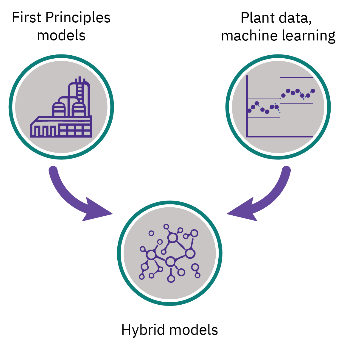
  First principles models

  Mass, momentum, and heat balances

• Empirical models

  Obtained by fitting experimental data.

  Statistical models

  Correlations

  data driven models

• Semi-empirical/ hybrid models

  A combination of the theoretical and empirical models

  The numerical values of one or more of the parameters in a theoretical model are calculated from experimental data.

Figure 7: Creating a hybrid model

Basic principles of mass and energy balances

• In general

  $$\begin{array}{}\text{(1)}& \text{accumulation}=\text{in}-\text{out}-\text{reaction}-\text{tranfer}\end{array}$$

• Mass balance (without reaction and transfer)

  $$\begin{array}{}\text{(2)}& \left\{\begin{array}{c}\text{rate of mass}\\ \text{accumulation}\end{array}\right\}=\left\{\begin{array}{c}\text{rate of}\\ \text{mass in}\end{array}\right\}-\left\{\begin{array}{c}\text{rate of}\\ \text{mass out}\end{array}\right\}\end{array}$$

• For component i (with reaction term included)

  $$\begin{array}{}\text{(3)}& \left\{\begin{array}{c}\text{rate of}\\ \text{component i}\\ \text{accumulation}\end{array}\right\}=\left\{\begin{array}{c}\text{rate of}\\ \text{component i}\\ \text{in}\end{array}\right\}-\left\{\begin{array}{c}\text{rate of}\\ \text{componenti }\\ \text{out}\end{array}\right\}+\left\{\begin{array}{c}\text{rate of}\\ \text{component i}\\ \text{produced}\end{array}\right\}\end{array}$$

Basic principles of mass and energy balances

• Energy balance

$$\begin{array}{}\text{(4)}& \begin{array}{rl}\left\{\begin{array}{c}\text{ rate of energy }\\ \text{ accumulation }\end{array}\right\}& =\left\{\begin{array}{c}\text{ rate of energy in }\\ \text{ by convection }\end{array}\right\}\\ & -\left\{\begin{array}{c}\text{ rate of energy out }\\ \text{ by convection }\end{array}\right\}\\ & +\left\{\begin{array}{c}\text{ net rate of heat addition }\\ \text{ to the system from }\\ \text{ the surroundings }\end{array}\right\}\\ & +\left\{\begin{array}{c}\text{ net rate of work }\\ \text{ performed on the system }\\ \text{ by the surroundings }\end{array}\right\}\end{array}\end{array}$$

Blending of two components

Figure 8: Stirred tank blending process

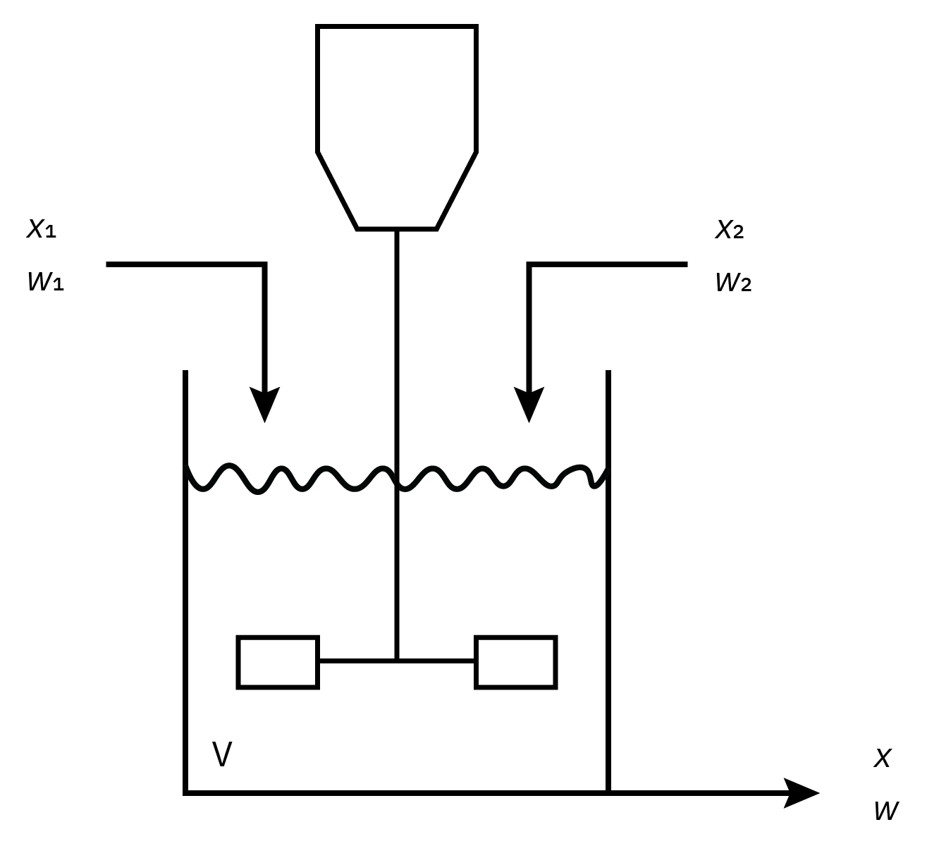
• Overall mass balance

  $$\begin{array}{}\text{(5)}& \left\{\begin{array}{c}\text{rate of accumulation}\\ \text{of mass in the tank}\end{array}\right\}=\left\{\begin{array}{c}\text{rate of}\\ \text{mass in}\end{array}\right\}-\left\{\begin{array}{c}\text{rate of}\\ \text{mass out}\end{array}\right\}\end{array}$$

  $$\begin{array}{}\text{(6)}& \frac{d(V\rho )}{dt}=w_1+w_2-w\end{array}$$

• Component balance

  $$\begin{array}{}\text{(7)}& \frac{d(V\rho x)}{dt}=w_1{x}_1+w_2{x}_2-wx\end{array}$$

It is possible to further simplify the system of two differential equations to

$$\begin{array}{}\text{(8)}& \frac{dV}{dt}=\frac{1}{\rho }(w_1+w_2-w)\end{array}$$

$$\begin{array}{}\text{(9)}& \frac{dx}{dt}=\frac{w_1}{V\rho }(x_1-x)+\frac{w_2}{V\rho }(x_2-x)\end{array}$$

Degrees of freedom (DOF) analysis

To simulate a process, it’s crucial to confirm that the model equations, both differential and algebraic, form a set of relations that can be solved. In simple terms, we need to ensure that the output variables (usually those on the left side of the equations) can be determined based on the input variables (those on the right side of the equations). For instance, consider a set of linear algebraic equations represented as y = Ax. To have a unique solution for x, vectors x and y need to have the same number of elements and matrix A should be nonsingular, meaning it has a nonzero determinant.

For large, complex steady-state or dynamic models, evaluating such a condition is not straightforward. However, a general requirement exists: for the model to have a unique solution, the count of unknown variables should match the number of independent model equations. In other words, all available degrees of freedom must be taken into account. The number of degrees of freedom, represented as $N_F$, can be determined using a particular expression.

$$\begin{array}{}\text{(10)}& N_F=N_V-N_E\end{array}$$

where $N_V$ is the total number of process variables (distinct from constant process parameters) and $N_E$ is the number of independent equations.

A degrees of freedom analysis allows modeling problems to be classified according to the following categories:

1. $N_F=0$: The process model is exactly specified. If $NF=0$, then the number of equations is equal to the number of process variables and the set of equations has a solution. (However, the solution may not be unique for a set of nonlinear equations.)

2. $N_F>0$: The process is underspecified. If $N_F>0$, then $N_V>N_E$, so there are more process variables than equations. Consequently, the $N_E$ equations have an infinite number of solutions, because NF process variables can be specified arbitrarily.

3. $N_F<0$: The process model is overspecified. For $N_F<0$, there are fewer process variables than equations, and consequently the set of equations has no solution.

DOF for the blending problem

• Parameters (2): $V,\rho$
• Variables ($N_V$ = 4): $x,x_1,x_2,w_1,w_1$
• equation ($N_E$ = 1): Equation 6

The degrees of freedom are calculated as $N_F=4-1=3$. Thus, we must identify three input variables that can be specified as known functions of time in order for the equation to have a unique solution. The dependent variable $x$ is an obvious choice for the output variable in this simple example. Consequently, we have

• output (1): $x$
• inputs (3): $x_1,w_1,w_2$

Because all of the degrees of freedom have been utilized, the single equation is exactly specified and can be solved.

Linearization of process models

Chemical processes often present nonlinear characteristics, leading to the creation of nonlinear ordinary differential equations (ODEs) through the modeling methods discussed in Chapter 4. However, these models can be complex and challenging, particularly when it comes to finding closed-form or analytical solutions. In addition, as we’ve seen in Chapter 3, straightforward input-output (I/O) representations can be highly beneficial for control engineers, making the control problem more discernible and aiding in the formulation of effective solutions.

Over time, control theory has evolved with a strong focus on linear systems, with a wealth of tools and methods available for designing and evaluating control systems. However, is it feasible to settle for a compromise in this case? There are many scenarios in which nonlinear processes predominantly operate around a specific point, meaning that a linear approximation of the process model in that vicinity may provide a satisfactory level of accuracy. These localized models can offer valuable insights into the problem at hand and aid in devising pragmatic control strategies. In this chapter, we begin by exploring how process models described by nonlinear differential equations can be linearly approximated.

To assist in constructing I/O relationships from linear models, we introduce the Laplace transform. A significant advantage of this transform is its ability to change linear differential equations into algebraic equations, greatly simplifying the mathematical manipulations needed to develop an I/O model. Such an algebraic model, known as the transfer function, is used extensively in control system design and analysis.

Figure 9: Laplace transform concept

Empirical models

• We can construct an empirical model using plant data

• Assume a certain idealized model structure

• First-order plus deadtime (FOPDT) model

  Time domain form $${\tau }_p\frac{dy(t)}{dt}+y(t)=K_{p}u(t-{\theta }_p)$$

  Frequency domain form (transfer function) $$G_p(s)=\frac{K_p{e}^{-{\theta }_{p}s}}{{\tau }_{p}s+1}$$

• $K_p$: Process gain; ${\tau }_p$: time constant; ${\theta }_p$: deadtime

FOPDT model is often used in controller tuning. A transfer function is a mathematical formula that describes how a system responds to different inputs over time.

Second-Order plus Deadtime (SOPDT) Model

• Time domain

  $${\tau }^2\frac{d^{2}y(t)}{d{t}^2}+2\xi \tau \frac{dy(t)}{dt}+y(t)=K_{p}u(t)$$

• Frequency domain

  $$G_p(s)=\frac{Y(s)}{U(s)}=\frac{K_p}{{\tau }^2{s}^2+2\xi \tau s+1}$$

• $K_p$: Process gain; $\tau$: time constant; $\xi$: damping factor or coefficient

• Behavior:

$\xi >1$: Overdamped

$0<\xi <1$: Underdamped

$\xi =1$: Critically damped

$\xi =0$: Sustained oscillations

$\xi <0$: Unstable

Dynamic Behavior of Processes

Input types

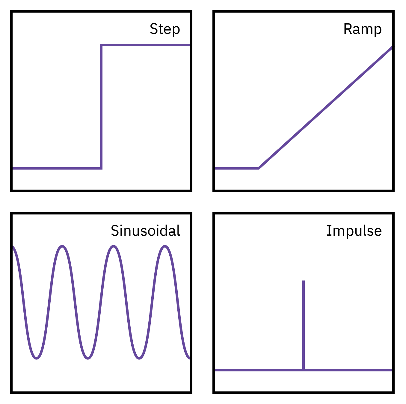
Figure 10: Input types

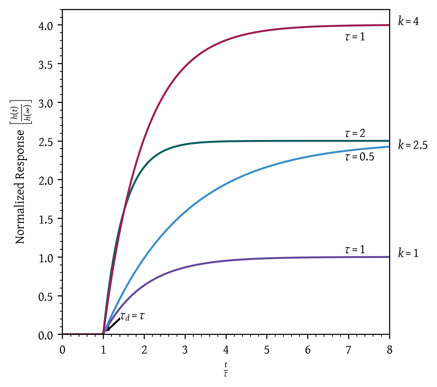
Response of first-order systems

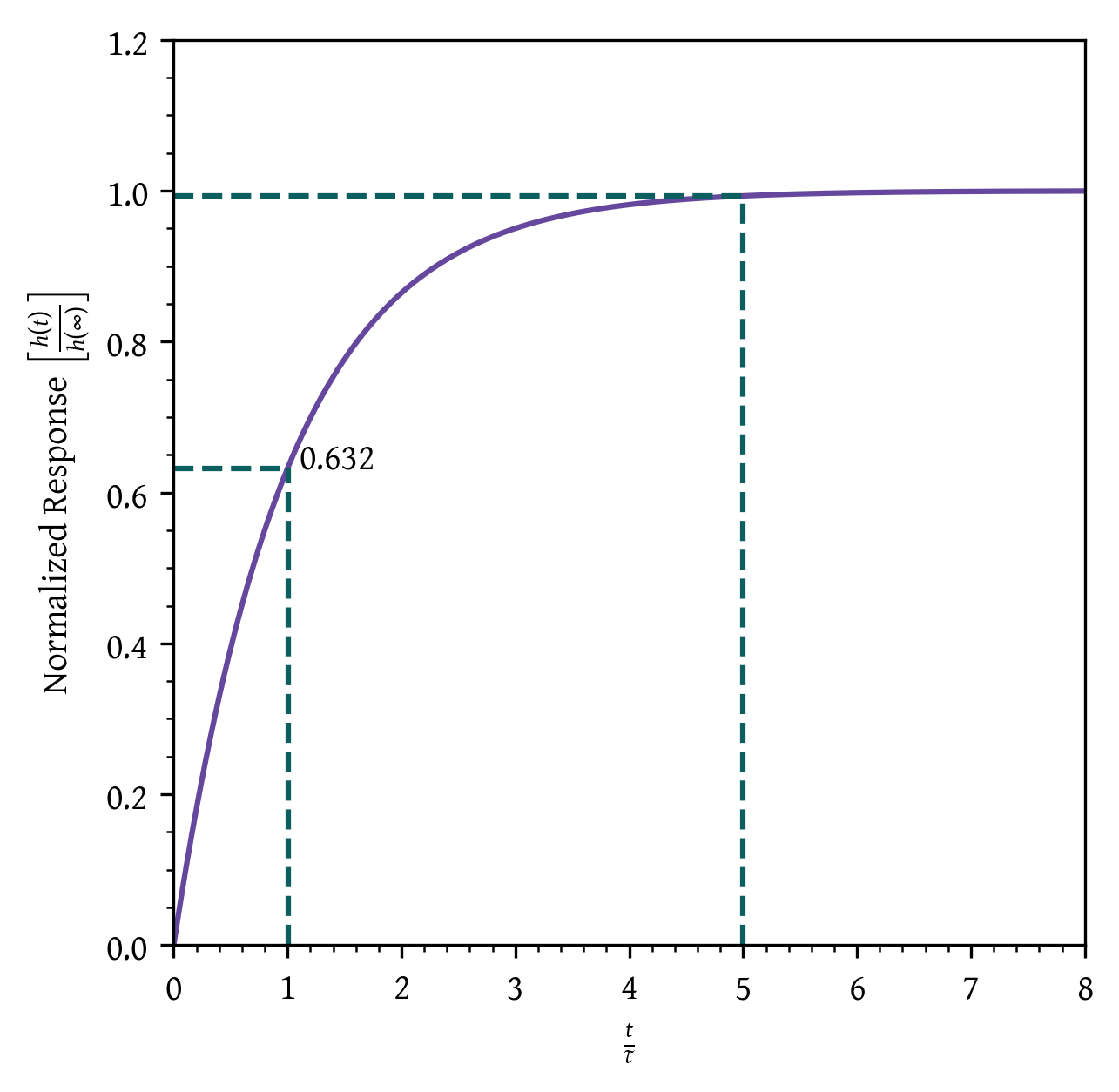
• The ultimate (steady-state) value of the response, $\overline{h}(t\to \mathrm{\infty })$, is equal to k for a unit-step change.

• When the elapsed time is equal to the process time constant $t=\tau$, the system reaches 63.2% of its final response.

• After approximately 5τ, the transient response can be considered as having reached steady-state.

• For a given t / τ, the output reaches the same fraction of the ultimate output response value.

In a tank process, a rise in the inlet flow rate elevates the liquid level, which in turn increases the hydrostatic pressure and subsequently the outlet flow rate. The system eventually reaches a new steady state. This feature is termed ‘self-regulation’.

Response of first-order systems

Response of second-order systems

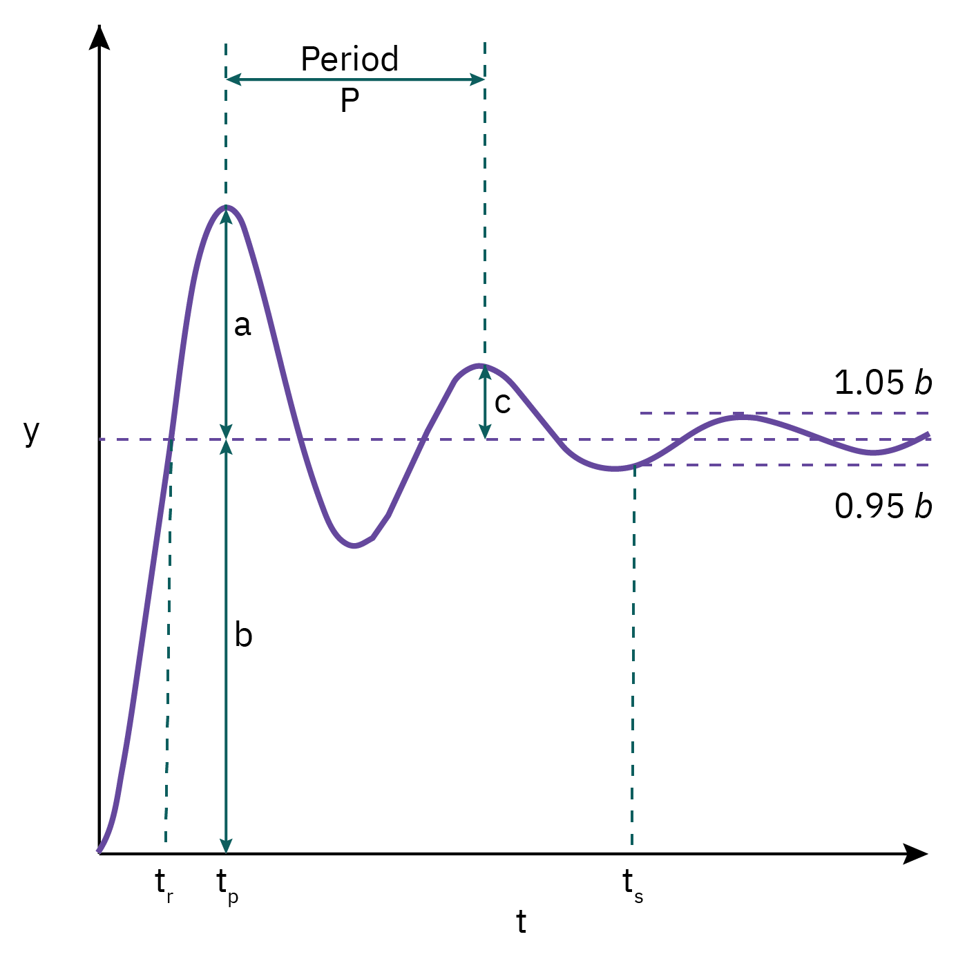
• Rise time ($t_r$): time required for y(t) to first cross its new steady state value

• Overshoot (a/b): The maximum amount by which the response exceeds the new steady state value

• Decay ratio (c/a): Ratio of the height of successive peaks in the response

• Period of oscillation (P): time for a complete cycle

• Response/ settling time ($t_s$): time required for the response to remain within a ± 5% band based upon steady state value.

Decay ratio, overshoot, response time, and damping factor (ξ) can be used as a basis for tuning.

Response of second-order systems

Critically damped (ξ = 1)

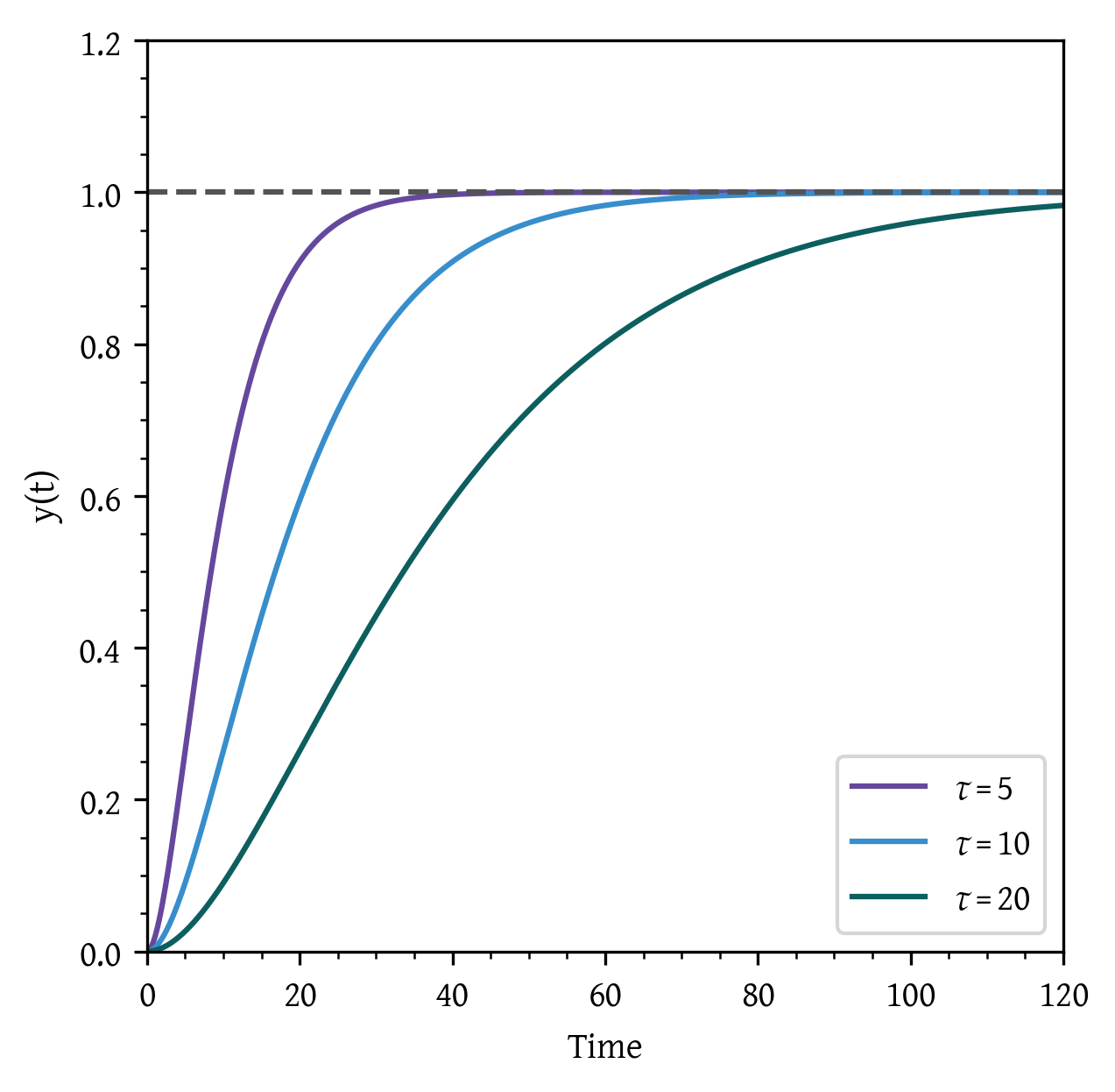
• Output response becomes more sluggish as τ increases.

• The responses are qualitatively similar.

Effect of ξ

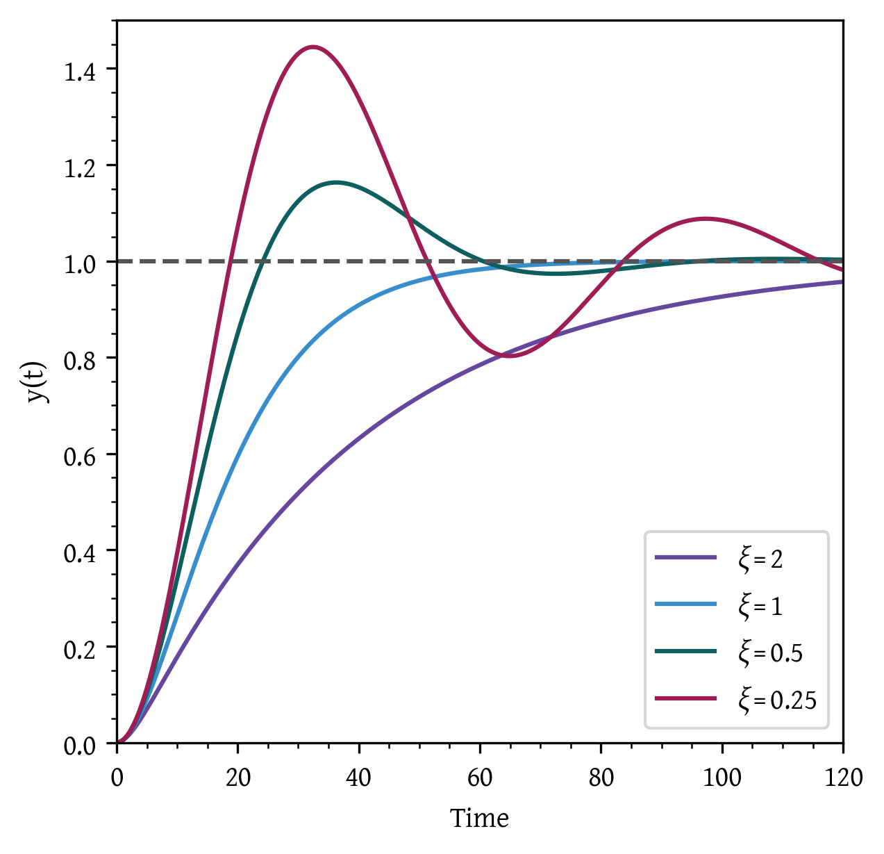
• ξ < 1: Oscillation and overshoot

• ξ > 1: Sluggish response, no oscillations; no overshoot

• ξ = 1: Fastest response, no oscillations; no overshoot

Analysis of Process Systems

• Stability analysis and the concept of poles and zeros
• Frequency response analysis
• Bode plots and Nyquist plots

Properties of transfer functions

• For transfer function

  $$g(s)=\frac{y(s)}{u(s)}=\frac{b_0{s}^m+\dots +b_m}{a_0{s}^n+\dots +a_n}=\frac{z(s)}{p(s)}$$

• The roots of the polynomial z(s) are the zeros of the transfer function or the zeros of the process.

• The roots of the polynomial p(s) are the poles of the transfer function or the poles of the process.

• A physical system needs to be proper ($n\ge m$), and casual (output depends only on past inputs)

• Characteristic equation

  The denominator polynomial p(s) when equated to zero is called the characteristic equation:

  $p(s)=a_0{s}^n+\dots +a_n=0$

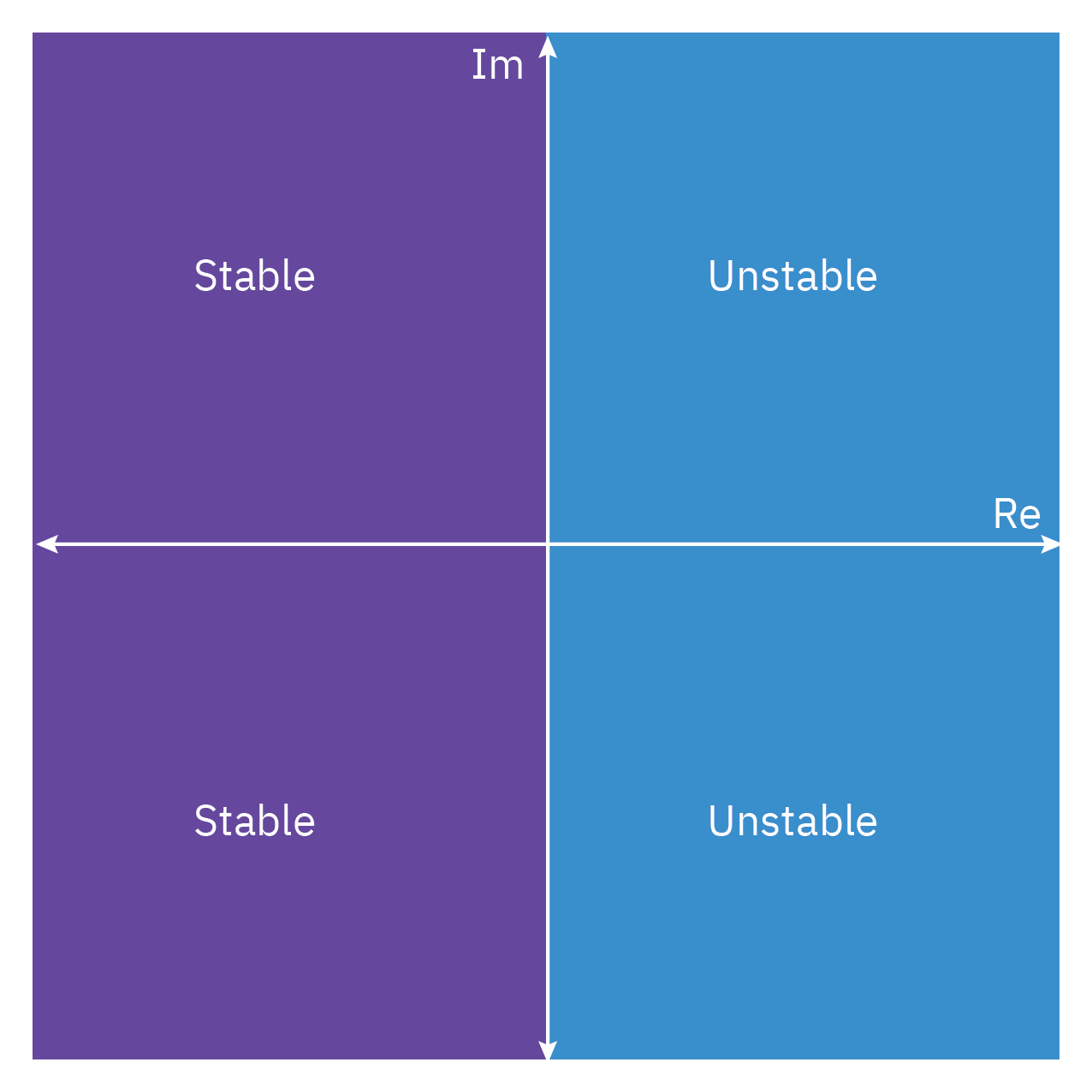
Stability of linear systems

• The location of the poles of a transfer function determines the bounded input–bounded output (BIBO) stability of a process.

• If the transfer function of a dynamic process has a pole with a positive real part, the process is unstable. If the real part is zero, then the process is critically stable

• We need to be cautious when we derive a transfer function model from a statespace model, because a zero (or zeros) may cancel a pole (or poles). This becomes especially important if the canceled pole is unstable, which means that those modes of the process would be hidden from us.

Routh’s Stability Criterion

Routh’s Criterion is a mathematical test that is used to determine whether a linear system is stable or unstable. It does not require explicit calculation of the roots of the characteristic equation.

• The first step in Routh’s Criterion is to set up the Routh array.

• Then, we examine the first column of the array. If there are no sign changes in the first column, the system is stable.

• If there are sign changes in the first column, the system is unstable. The number of sign changes corresponds to the number of roots with positive real parts.

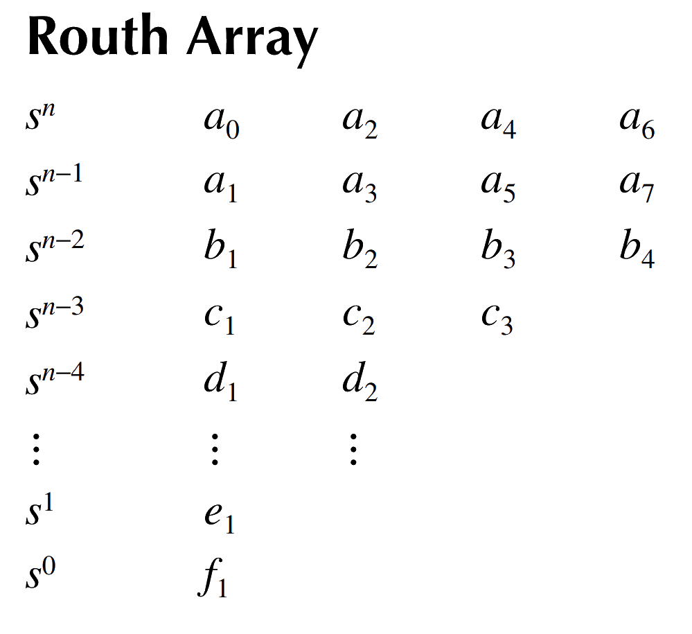
Routh’s Criterion can also be used to determine relative stability and system type.

Root locus method

Root Locus is a graphical method used in control systems to examine how the system stability changes with varying gain.

• It shows possible pole locations as system gain varies from zero to infinity.

• The method provides insights into stability and transient response.

• Root locus begins at open-loop poles and ends at open-loop zeros.

• The plot exists on parts of the complex plane where the number of open-loop poles and zeros to the right is odd.

• Consider the characteristic equation $$p(s,k)=s^2+s+k=0$$

D:\Users\Ranjeet\vault\work\teaching\CHEN4011 Advanced Modeling and Control\2025_S2\content\.venv\Lib\site-packages\control\ctrlplot.py:164: FutureWarning: return of Line2D objects from plot function is deprecated in favor of ControlPlot; use out.lines to access Line2D objects
  warnings.warn(
Ignoring fixed x limits to fulfill fixed data aspect with adjustable data limits.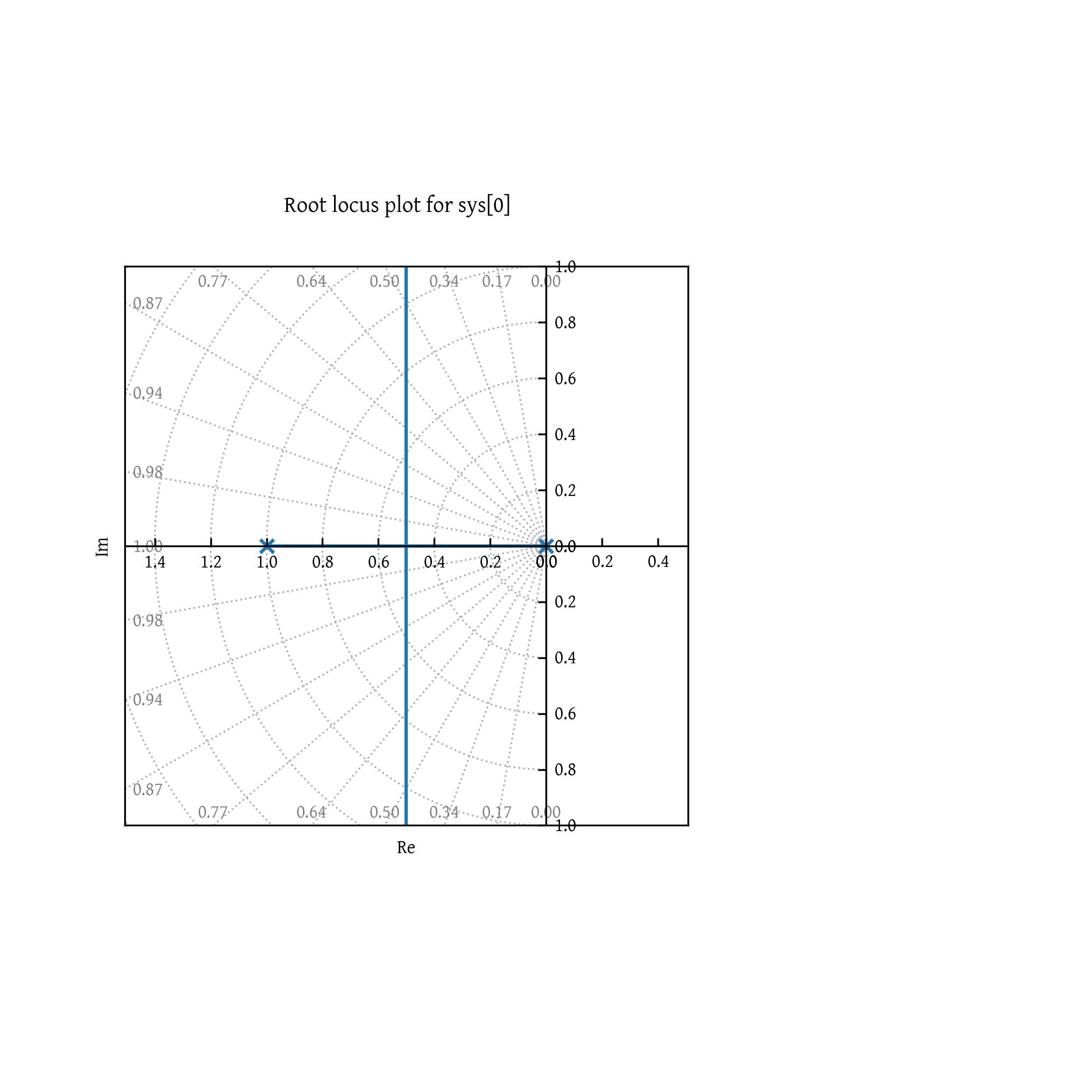

Frequency response analysis

Bode plots and Nyquist plots

Introduction to feedback control

Proportional, integral, and derivative control actions

PID control and tuning methods

Stability analysis

Seborg, Dale E., Thomas F. Edgar, Duncan A. Mellichamp, and Francis J. Doyle III. 2016. Process Dynamics and Control. John Wiley & Sons. https://books.google.com?id=ZZVFEAAAQBAJ.