AMC | Advanced Modeling and Control – Introduction to digital control

Introduction

Use of digital computers or microcontrollers to manage the behavior of dynamic systems.
Typically includes
- sampling an analog signal
- processing the data in discrete steps (using algorithms or controllers like PID), and
- generating a control signal to influence the system.
Benefits: programmability, flexibility, computational power, improved precision over analog control systems.
Key components
- analog-to-digital converters (ADCs)
- digital-to-analog converters (DACs)
- and software for processing the control logic.

Discrete control

Continuous control systems: signals are processed continuously over time,
Discrete control systems:
- Managing dynamic systems using digital signals sampled at specific time intervals.
- Work with signals at discrete moments, dictated by a sampling period.
Sampling: Converting a continuous signal into a sequence of discrete values at regular intervals.
Quantization: Representing the sampled values in a digital form.
Control Logic: Using algorithms like PID or state-space models to make decisions based on the discrete samples.
Actuation: Producing a control signal that affects the system’s behavior.

z-transform

Discrete-time counterpart of the Laplace transform
Converts a discrete-time signal (sequence of numbers) into a complex frequency domain representation.

Definition

The z-transform of a discrete-time signal $x[n]$ is defined as:

$X(z) = \sum_{n=-\infty}^{\infty} x[n] z^{-n}$

where:

$x[n]$ is the discrete-time signal (sequence).
$n$ is the discrete-time index (integer).
$z$ is a complex variable, defined as $z = r e^{j\omega}$ , where $r$ is the radius and $\omega$ is the angle in radians.

Relationship between z-plane with s-plane

Processes are stable if they do not possess the poles that lies outside the unit-circle in the z-plane.

z-transform

Function sampled at discrete time step $T_s$

$f(nT_s) = \begin{cases} f(t) & \text{for } n = 0, 1, 2, \ldots \\ 0 & \text{otherwise} \end{cases} = f^(t)$
Laplace transform of $f(t)$ : $F(s) = \int_{0}^{\infty} e^{-st} f(t) \, dt$
We can also apply Laplace transform to $f^(t)$ : $F^(s) = \int_{0}^{\infty} e^{-st} f^(t) \, dt$
Since $f^(t)$ only exists at sampling instant

$F^(s) = \sum_{n=0}^{\infty} f(nT) e^{-nsT}$
Defining $z = e^{sT}$

$F^(s) = \sum_{n=0}^{\infty} f(nT) e^{-nsT} = \sum_{n=0}^{\infty} f(nT) z^{-n} = F(z)$

z-transform

Exists only if the summation of infinite terms takes finite values. Depends on sampling period T
z-transform is merely a Laplace transform for a sampled data sequence, as such inherits many of the properties of Laplace transform.
z-transform allows:
- Development of input-output models for discrete-time system
- Can be used to analyze how discrete-time processes react to external input changes.

z-transform

z-transform of unit step

$Z[\text{Unit Step}] = \frac{z}{z-1}$
z-transform of the discrete cosine signal

$Z[\cos \omega t] = \frac{z^2 - z \cos \omega t}{z^2 - 2z \cos \omega t + 1}$
If $\omega t = 2n\pi = nT$ ,

$Z[\cos (nT)] = \frac{z^2 - z}{z^2 - 2z + 1} = \frac{z}{z-1}$
The values of a unit step function and cosine wave sampled at uniform intervals of period T are the same.
Impossible to distinguish two functions, which have the same samples values at the sampling instants.

Aliasing

Different continuous-time signals can produce the same set of samples if the sampling rate is not appropriately chosen
- The sampling process cannot capture frequencies higher than half the sampling rate (the Nyquist rate).
If two signals sampled at uniform intervals have the same values, they are indistinguishable when only looking at their samples.
- The resulting discrete-time sequence may not uniquely identify the original continuous-time signal.
- Loss of information during the sampling process
- Errors in signal processing and control applications

Nyquist-Shannon sampling theorem

To avoid aliasing, the sampling rate must be at least twice the highest frequency component of the signal being sampled. Failing to do so can cause the overlap of spectral components, resulting in different signals becoming indistinguishable.

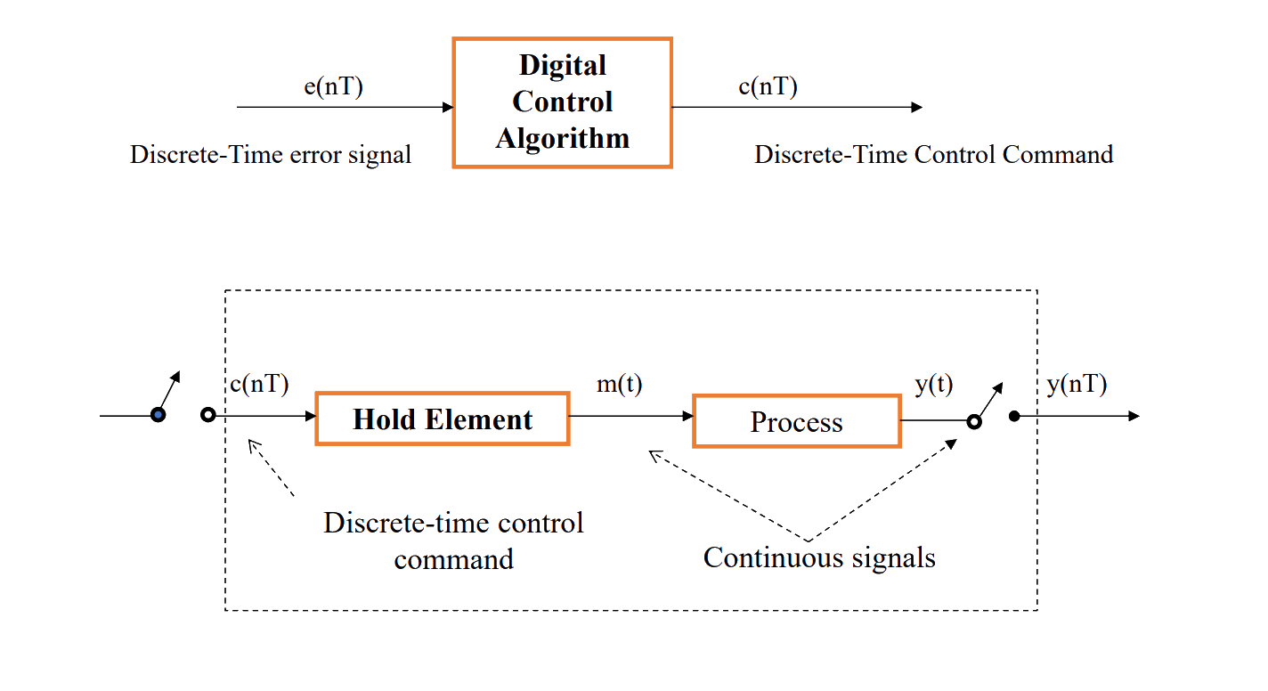
Direct digital control (DDC)

Two Primary Components:
- Digital Control Algorithm: A discrete component responsible for processing the error and generating control commands in discrete-time.
- Process with Hold Elements: The hold elements convert the discrete-time control commands into continuous signals, enabling interaction with a continuous-time process (plant).

Discrete time analysis

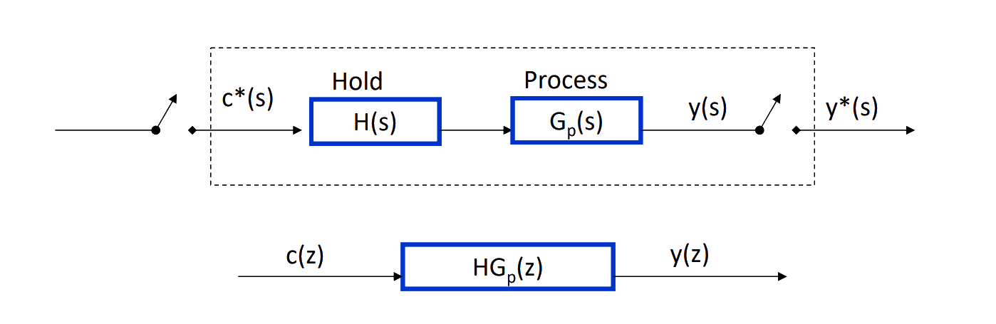
The pulse transfer function relates the discrete-time output $y(nT)$ to the discrete-time control command $c(nT)$ using z-transforms.
The system components consist of the hold element $H(s)$ and the process $G_p(s)$ , combined as:

$H(s) G_p(s)$
The z-transform is applied to obtain the equivalent transfer function in the z-domain: $\frac{Y(z)}{C(z)} = H G_p(z) = \mathcal{Z} \{ H(s) G_p(s) \}$

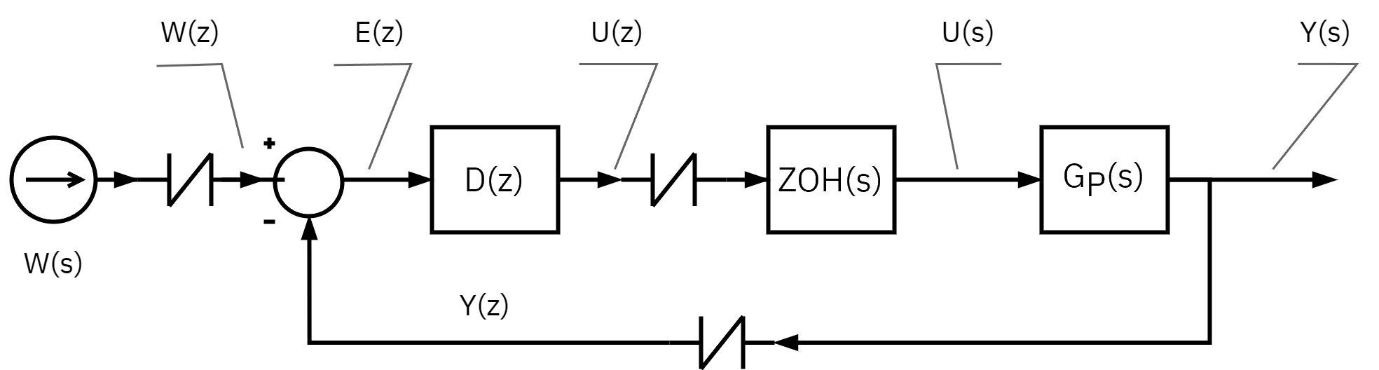
Block diagram manipulation

Manipulation of block diagrams of sampled data systems are very similar to that for those in the Laplace domain.
The z-transform is a special case of the Laplace transform.
The presence of samplers, there are some extra rules to follow
ZOH denotes zero-order hold element

z-transform of continuous-time transfer functions

System A

$Y(z) = \mathcal{Z} \{ F(s) \} \cdot \mathcal{Z} \{ G(s) \} \cdot U(z)$

$Y(z) = F(z)G(z)U(z)$

Discretizes each transfer function separately and then multiplies them in the z-domain.

System B

$Y(z) = \mathcal{Z} \{ F(s)G(s) \} \cdot U(z)$

$Y(z) = FG(z)U(z)$

First combines the transfer functions in the ( s )-domain and then applies the z-transform

The order of discretization and multiplication matters.
Applying the z-transform separately to each transfer function is generally not equivalent to applying the z-transform to the combined transfer function in the s-domain.

MATLAB functions

MATLAB built-in function to convert a continuous transfer function G(s) to discrete system cdc
- SYSD = c2d(SYSC,TS,METHOD) computes a discrete-time model SYSD with
sample time TS that approximates the continuous-time model SYSC.

The string METHOD selects the discretization method among the following:
- zoh - Zero-order hold on the inputs
- foh - Linear interpolation of inputs
- impulse - Impulse-invariant discretization
- tustin - Bilinear (Tustin) approximation.
- matched - Matched pole-zero method (for SISO systems only).
- least-squares - Least-squares minimization of the error between frequency responses of the continuous and discrete systems (for SISO systems only).

Effect of sampling period

Long sampling period leads to slower response compared to the continuous PI controller
Smaller sampling period leads to faster response and approaching that of the continuous PI controller as the sampling period decreases
In practice, there is a trade-off between short sampling period and storage/computational capacity
Short sampling period requires more computational and storage capacity but gives good control performance
Long sampling period requires less storage and computational capacity but lower control performance

Position form of a PID controller

Discrete implementation of the PID control law where the controller output is updated at each sampling time.
At each sampling time the actual value (position) of the output signal is calculated based on the current error and its historical behavior.
The PI controller saves:
- Current Error $e_n$
- Sum of All Previous Errors $S_{n-1}$ : $S_{n-1} = \sum_{i=1}^{n-1} e_i$
PI Control Law

$c_n = K_c \left[ e_n + \frac{T}{\tau_I} (S_{n-1} + e_n) \right] + c_s$
PID Controller

$c_n = K_c \left[ e_n + \frac{T}{\tau_I} (S_{n-1} + e_n) + \frac{\tau_D}{T} (e_n - e_{n-1}) \right] + c_s$
- PID saves previous errors as well

Velocity form of a PID controller

Focuses on calculating the change in the controller output at each sampling time rather than the absolute position (total output).
Instead of directly calculating the full controller output, the velocity form computes the change in output ( $\Delta c_n$ ) between successive sampling times $n$ and $n-1$ .
At the $n$ -th sampling period $c_n = K_c \left[ e_n + \frac{T}{\tau_I} \sum_{k=0}^n e_k + \frac{\tau_D}{T} (e_n - e_{n-1}) \right] + c_s$
At the $(n-1)$ -th sampling period $c_{n-1} = K_c \left[ e_{n-1} + \frac{T}{\tau_I} \sum_{k=0}^{n-1} e_k + \frac{\tau_D}{T} (e_{n-1} - e_{n-2}) \right] + c_s$
The velocity form of the PID controller calculates the difference between $c_n$ and $c_{n-1}$ $\Delta c_n = c_n - c_{n-1} = K_c \left( \left[ 1 + \frac{T}{\tau_I} + \frac{\tau_D}{T} \right] e_n - \left[ 1 + \frac{2\tau_D}{T} \right] e_{n-1} + \frac{\tau_D}{T} e_{n-2} \right)$

Position vs velocity form

Aspect	Position form	Velocity form
Simplicity & Intuitiveness	Direct calculation of output; simpler	Calculates change in output; may be
	to understand and implement	less intuitive initially

Integral Action Handling	Full integral action for precise error	Limited integral effect to prevent
	elimination	windup

Response to Slow Dynamics	Works well in systems with slow dynamics	More responsive in fast systems

Memory & Computational	Suitable if memory isn’t a constraint	More efficient, lower memory
Load		requirement

Risk of Windup & Stability	Potential for windup; needs careful	Reduces windup and increases
	tuning	stability in saturated systems

Control Signal Saturation	Not optimized for saturation	Suitable for limited-range actuators;
		prevents large jumps

Conclusion

Digital control enhances flexibility, precision, and easy implementation of algorithms.
Understanding the s-plane to z-plane relationship is key for stable discrete system design.
The sampling period impacts performance; shorter periods improve control but increase computation.
Proper sampling rates prevent aliasing, ensuring accurate discrete-time signal representation.
DDC bridges digital algorithms and continuous processes effectively using hold elements.
Position and velocity PID forms suit different needs based on system dynamics and computational trade-offs.