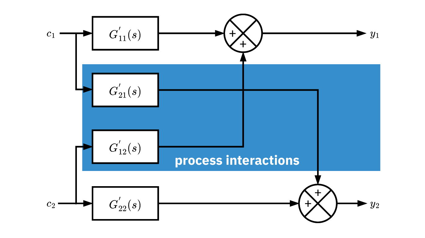
AMC | Advanced Modeling and Control – Multivariable Centralized Control and MPC

2x2 MIMO process system

Inputs: $c_1, c_2$ . Outputs: $y_1, y_2$ .
Plant ransfer function matrix
$\mathbf{G}=\begin{bmatrix} G'_{11} & G'_{12} \\ G'_{21} & G'_{22} \end{bmatrix}$
$G'_{12}$ is the transfer from $c_2$ to $y_1$ .
Interactions: a change in $c_1$ or $c_2$ affects both outputs.
Cross terms $G'_{12}$ and $G'_{21}$ create loop coupling.
Interactions can limit decentralized control performance.

Decoupler can be used to reduce the coupling effect
Model predictive control (MPC)

Decoupling controller

A decoupling controller (decoupler) can be added to decentralized control
to reduce process interactions
Types of decoupling systems:
- Partial decoupling (one-way):
  
  Cancels the interaction in one direction
  
  Most common in practice
- Complete decoupling (two-way):
  
  Cancels interactions in both directions
  
  Useful for severe interactions but often requires very high control action
  
  Leads to increased valve wear and tear
A one-way decoupler is typically designed for a pair of control loops to
cancel the interaction from one loop to the other
Two decouplers can be used for the same pair of loops to cancel interactions
in both directions

One way decoupler

Assume perfect cancellation of coupling effect from loop 2 to loop 1

$U_2 D_{12} G_{11} + U_2 G_{12} = 0$

$\therefore \; D_{12} = - \frac{G_{12}}{G_{11}}$

General equation for decoupler $D_{ij}$

$D_{ij} = - \frac{G_{ij}}{G_{ii}}$

$D_{ij}$ is used to remove the coupling effect from loop $j$ to loop $i$

Two way decoupler

For an $n \times n$ MIMO system, $n(n-1)$ decouplers are required in a complete decoupling system
Complete decoupling is often not practical for large MIMO systems
Partial decoupling is more commonly adopted

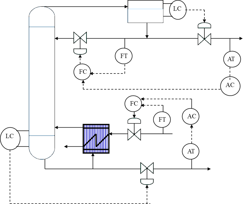
Multi-loop controllers for distillation column

A common application of multi-loop control is the control of a distillation column
There are 4 controlled variables:
- Liquid level in reflux drum
- Liquid level at the bottom of the column
- Top composition
- Bottom composition
This forms a $4 \times 4$ decentralized control system
Each loop employs an individual PID-type controller

Multivariable control (MPC)

For weak interactions and loose constraints, a simpler multi-loop PID
approach is often sufficient
Fast, lightly coupled units can run well with well-tuned SISO loops
In MIMO systems with strong interactions, multi-loop coordination becomes complex
Multivariable Predictive Control (MPC)
- Uses a process model to predict future behavior and choose control moves
  over a short horizon
- The controller optimizes, applies the first move, then repeats at the next
  sample
Compared with multi-loop PID, MPC considers all inputs and outputs together
and accounts for interactions
MPC enforces constraints on actuators and process variables explicitly
MPC looks ahead in time rather than reacting loop by loop
Advantages
- Better coordination when loops are strongly coupled
- Safer, more efficient operation under tight constraints
- Improved performance on processes with delays and slow dynamics

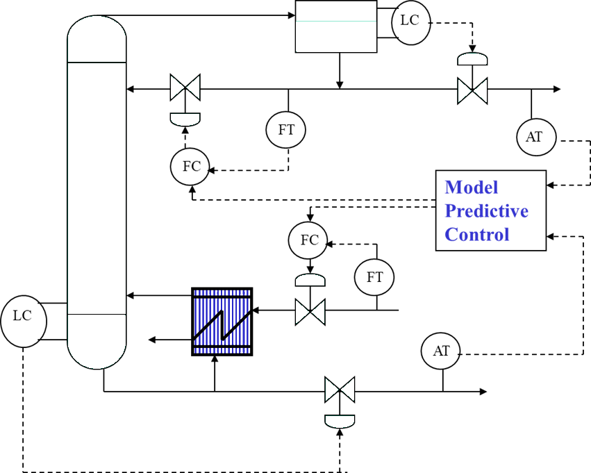
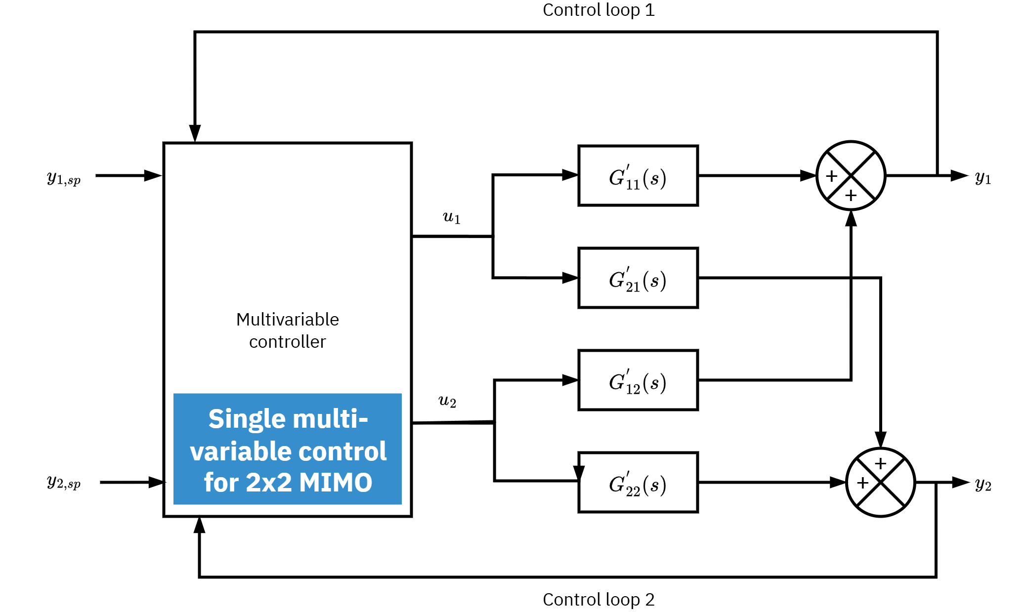
Multivariable controllers for distillation column

Replace the two SISO composition controllers with a single multivariable controller (MPC)
MPC reduces the negative effects of loop couplings between top and bottom compositions
Loop couplings are a major limitation to achievable control performance
Mixed control strategy:
- MPC for composition loops
- PID controllers for level loops
Keep level controllers as SISO since interactions between level loops are relatively small

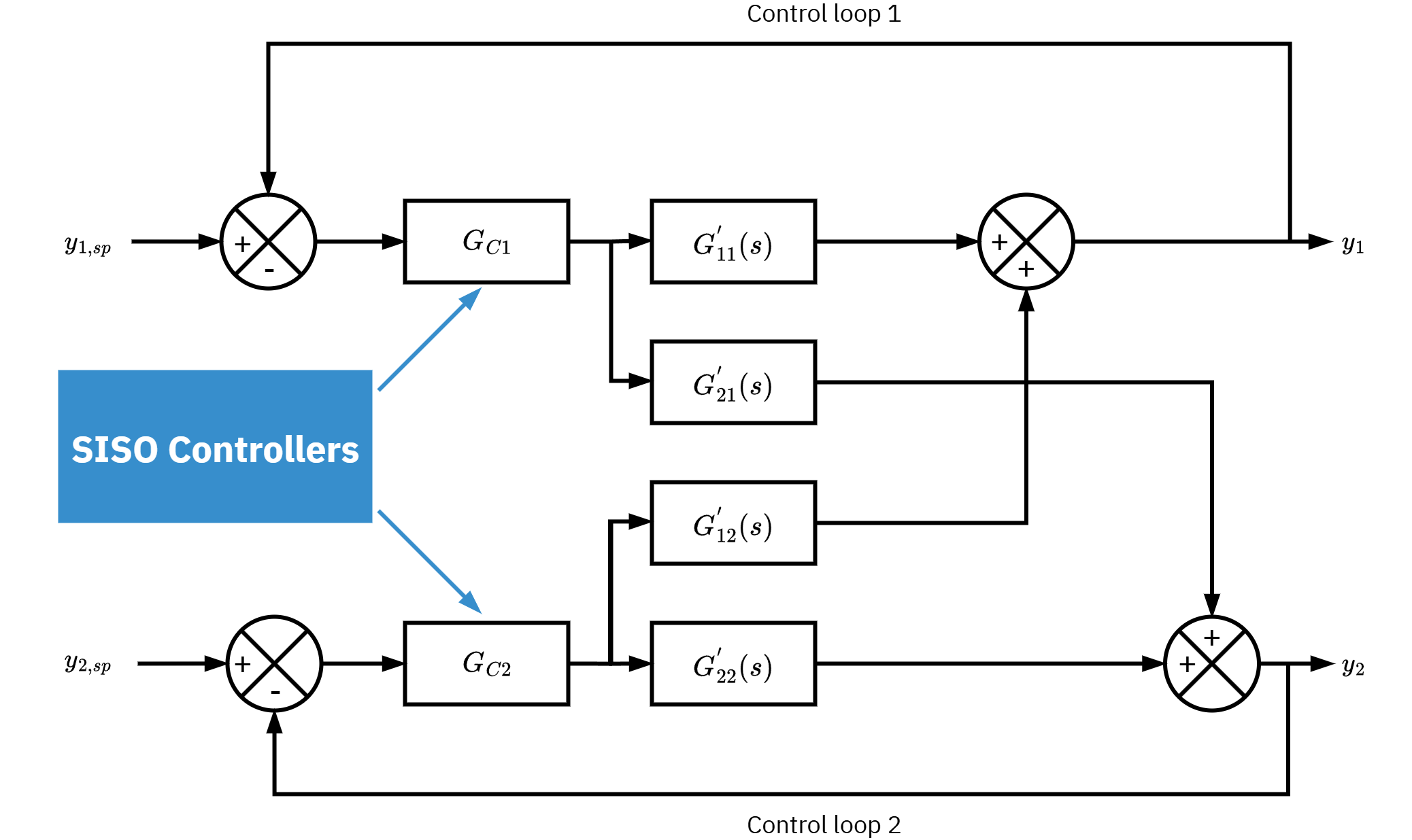
Multi-loop control block diagram

Multivariable controller block diagram

Model Predictive Control (MPC)

Overview

Widely used multivariable control approach in process industry
often considered the gold standard for coordinating interacting loops
Handles soft and hard constraints on inputs and outputs
Conventional PID cannot enforce constraints explicitly
Can operate close to economic or safety limits without violating constraints
Several industrial variants exist; dynamic matrix control (DMC) is the most common lineage

Advantages

Provides decoupling to reduce effects of process interactions
Enables feedforward compensation for measured disturbances
Can address process nonlinearity when a nonlinear model is used
Enforces constraints directly on variables and move rates

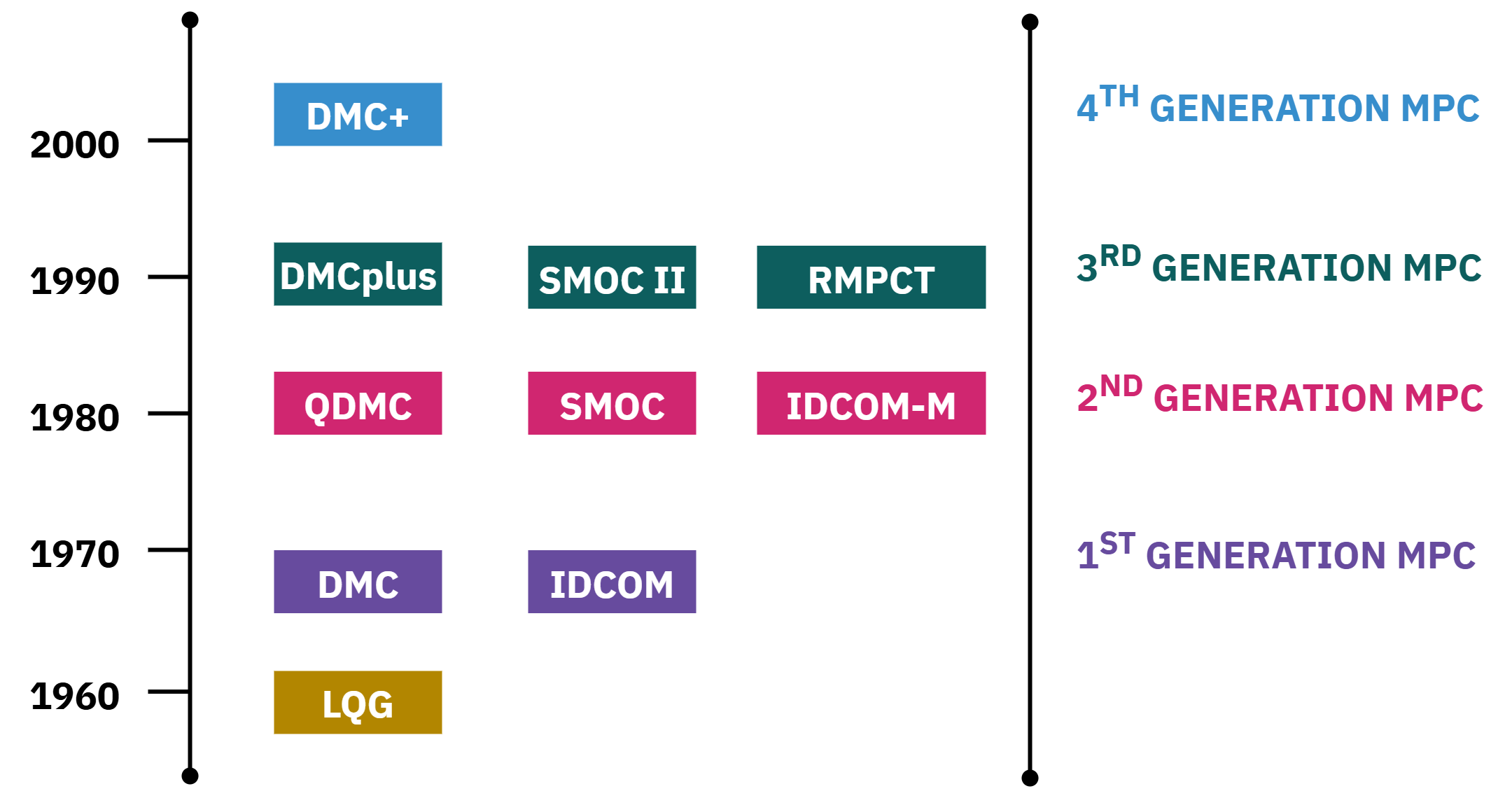
Genealogy of linear MPC algorithms

MPC emerged in the late 1970s and early 1980s, evolving from Linear Quadratic Gaussian (LQG) control introduced by Kalman in the 1960s
MPC performs prediction within a finite time horizon, unlike LQG which assumes infinite horizon and unconstrained optimization

1st generation (1970s)
- DMC: dynamic matrix control Shell implementations
- IDCOM: Texas Instruments multivariable controller
2nd generation (1980s)
- QDMC: quadratic dmc shell
- SMOC: setpoint multivariable optimal control
- IDCOM-M: multivariable extension
3rd generation (1990s)
- DMCPLUS: AspenTech commercial successor
- RMPCT: Honeywell robust MPC
- SMOC-II: Shell evolution
4th generation (2000s and onward)
- DMC+ enhanced commercial variants

Dynamic Matrix Control (DMC)

Developed by Shell Oil engineers and first applied in 1973
Based on a linear step response model of the plant
Uses a quadratic performance objective over a finite prediction horizon
Computes future control actions so the controlled variables follow setpoints as closely as possible
Became the first widely adopted form of model predictive control in the process industry

Discrete-Time Step Response Model (DTSRM)

Dynamic Matrix Control (DMC) requires a dynamic model of the process
DTSRM is the model structure used in DMC
Provides the basis for calculating optimal control actions
Equivalent to the transfer function model $G_p$ used in conventional control
Captures the effect of manipulated variables (MV) on controlled variables (CV)
Offers the same process information as $G_p$ but expressed in step response form

DTSRM developed from FOPDT

Start with a FOPDT model

$G_p(s) = \frac{y(s)}{u(s)} = \frac{\exp(-s)}{s+1}, \quad K_p = 1, \, \tau_p = 1, \, \theta_p = 1$

Apply a unit step change in input

$\Delta u(s) = \frac{1}{s} \quad \text{at } t = t_0$

Choose a fixed sampling time, e.g. $T_s = 1$
From the step test, derive DTSRM coefficients

$a_i = \frac{y'(i)}{\Delta u(t_0)}, \quad y'(i) = y(i) - y(0) \tag{1}$

A set of coefficients $a_i$ for $i = 0, 1, 2, \dots, n$ defines the DTSRM

Example: DTSRM

t	i	Δu	y(t)	aᵢ
0	0	1	0.00	0.00
1	1	0	0.00	0.00
2	2	0	0.63	0.63
3	3	0	0.87	0.87
4	4	0	0.95	0.95
5	5	0	0.98	0.98
6	6	0	0.99	0.99
7	7	0	1.00	1.00
8	8	0	1.00	1.00

Input step change at $t = 0$ by 1 unit
Only one input change is applied at $t = 0$
Several input changes could be applied at different $t$ values
A set of coefficients $a_i$ for $i = 0, 1, \dots, 8$ is calculated
$n$ is chosen so that the process reaches a new steady state

Response of a process to an input change

From Eqn. (1):

$y(t_i) = y'(t_i) + y(t_0) = a_i \Delta u(t_0) \tag{2}$

Eqn. (2) can be extended to predict $y(t)$ for several input changes at $t = t_0, t_1, t_2, \dots$

$\begin{cases} y_1 - y_0 = a_1 \Delta u_0 = a_1 \Delta u(t_0) \\ y_2 - y_0 = a_2 \Delta u_0 + a_1 \Delta u_1 \\ y_3 - y_0 = a_3 \Delta u_0 + a_2 \Delta u_1 + a_1 \Delta u_3 \end{cases} \tag{3}$

In general:

$y_n - y_0 = \sum_{i=1}^{n} a_i \Delta u(t_{n-i}) \tag{4}$

Response to input changes in matrix form

$\begin{bmatrix} y'(t_1) \\ y'(t_2) \\ y'(t_3) \\ y'(t_4) \\ \vdots \\ y'(t_n) \end{bmatrix} = \begin{bmatrix} a_1 & 0 & 0 & 0 & \cdots \\ a_2 & a_1 & 0 & 0 & \cdots \\ a_3 & a_2 & a_1 & 0 & \cdots \\ a_4 & a_3 & a_2 & a_1 & \cdots \\ \vdots & \vdots & \vdots & \vdots & \ddots \\ a_m & a_{m-1} & \cdots & a_2 & a_1 \end{bmatrix} \begin{bmatrix} \Delta u(t_0) \\ \Delta u(t_1) \\ \Delta u(t_2) \\ \Delta u(t_3) \\ \vdots \\ \Delta u(t_{n-1}) \end{bmatrix}$

$y' = A \Delta u$

$n$ is the prediction horizon
$m$ is the model horizon
$n > m$ , typically $n = 1.5m$
For a single input step change: $T_{stt} = mT_s$
For multiple input changes, settling time is longer than $T_{stt}$

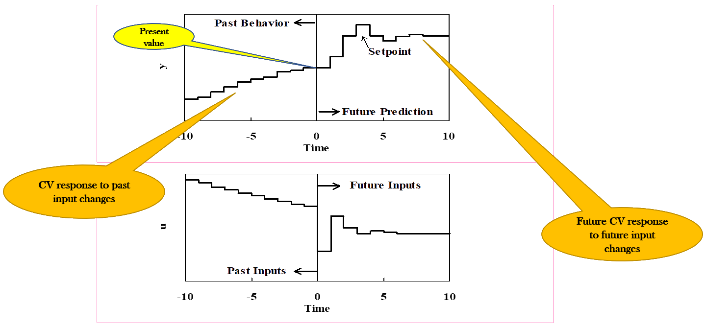
Moving horizon algorithm

Future manipulated variable (MV) values are chosen to regulate the controlled variable (CV) to its setpoint using the DTSRM and past input history
After each control interval, the present CV value and the last MV change $\Delta u(t)$ are measured
The controller recalculates a new sequence of MV values into the future to meet the control objective
Only the first move from the optimized sequence is implemented
- At the next interval, the horizon shifts forward and the optimization is repeated

Prediction vector $y^P$

So far, we assumed that $y(t_0)$ is at steady state and MV changes occur only for $t > t_0$
In practice, this assumption is unrealistic since MV changes for $t < t_0$ are likely to exist
The effect of past input changes $\Delta u(t)$ for $t < t_0$ must be included to predict future CV behavior
The prediction vector $y^P$ represents the effect of previous MV changes on CV for $t > t_0$
- If no future MV changes are applied ( $\Delta u(t) = 0$ for $t > t_0$ ), $y^P$ captures the continuing response of the CV

Prediction vector $y^P$

Assume the model horizon $m$ time steps, so that an input change has reached steady state
Using Eqn. (4), the prediction vector at $t = t_1$ is

$\begin{aligned} y^P(t_1) = \; & y(t_{-m}) + a_m \Delta u(t_{-m}) + a_m \Delta u(t_{-m+1}) \\ & + a_{m-1}\Delta u(t_{-m+2}) + \dots + a_2 \Delta u(t_{-1}) \end{aligned} \tag{5}$

Notes:
- $a_{-m} = a_m, \; a_{-m+1} = a_{m+1}, \dots$
- $a_{m+j} = a_m$ for $j = 1, 2, 3, \dots$ once the steady state is reached
- Negative subscripts indicate sampling intervals before $t_0$
General form:

$y^P(t_1) = y_{-m} + \sum_{i=-m}^{-1} a_i \Delta u(t_{m-i})$

Matrix form of $y^P$

$\begin{bmatrix} y^P(t_1) \\ y^P(t_2) \\ \vdots \\ y^P(t_n) \end{bmatrix} = \begin{bmatrix} y(t_{-m}) \\ y(t_{-m}) \\ \vdots \\ y(t_{-m}) \end{bmatrix} + A^P \begin{bmatrix} \Delta u(t_{-m}) \\ \Delta u(t_{-m+1}) \\ \vdots \\ \Delta u(t_{-1}) \end{bmatrix}$

$y^P = y(t_{-m}) + A^P \Delta u^P$

$n$ = prediction horizon (number of future steps, with $n > m$ )
$m$ = model horizon (time steps needed for steady-state response)
$y(t_{-k})$ = value of CV at $t = t_0 - kT_s$ , where $k$ is the number of steps from present to historical past

Prediction values of $y(t)$ for $t > t_0$

Future CV values are predicted by combining effects of:
- Past input movements (prediction vector $y^P$ )
- Future input movements ( $\Delta u$ )

$\tilde{y} = y^P + A \Delta u$

$\therefore \; \tilde{y} = y(t_{-m}) + A^P \Delta u^P + A \Delta u$

Accuracy of predictions depends on:
- Errors in identifying DTSRM coefficients
- Unmeasured disturbances
- Nonlinear process behavior
- Lack of steady-state behavior at $t = t_{-m}$

Reducing Effects of Process/Model Mismatch

Reliability of MPC requires that the deviation of the model from the actual process is small
- Large mismatch can degrade control performance
The error between measured $y(t_0)$ and predicted $y^P(t_0)$ can be used to correct predictions
Recall equation (6):
$\tilde{y} = y^P + A \Delta u$
Prediction error:
$\varepsilon = y^P(t_0) - y(t_0)$
Corrected model:
$y = y^P + A \Delta u + \phi^T$
Error vector:
$\phi = [\varepsilon, \varepsilon, \varepsilon, \dots, \varepsilon]$
Number of rows of $\phi^T$ matches the dimension of $y$

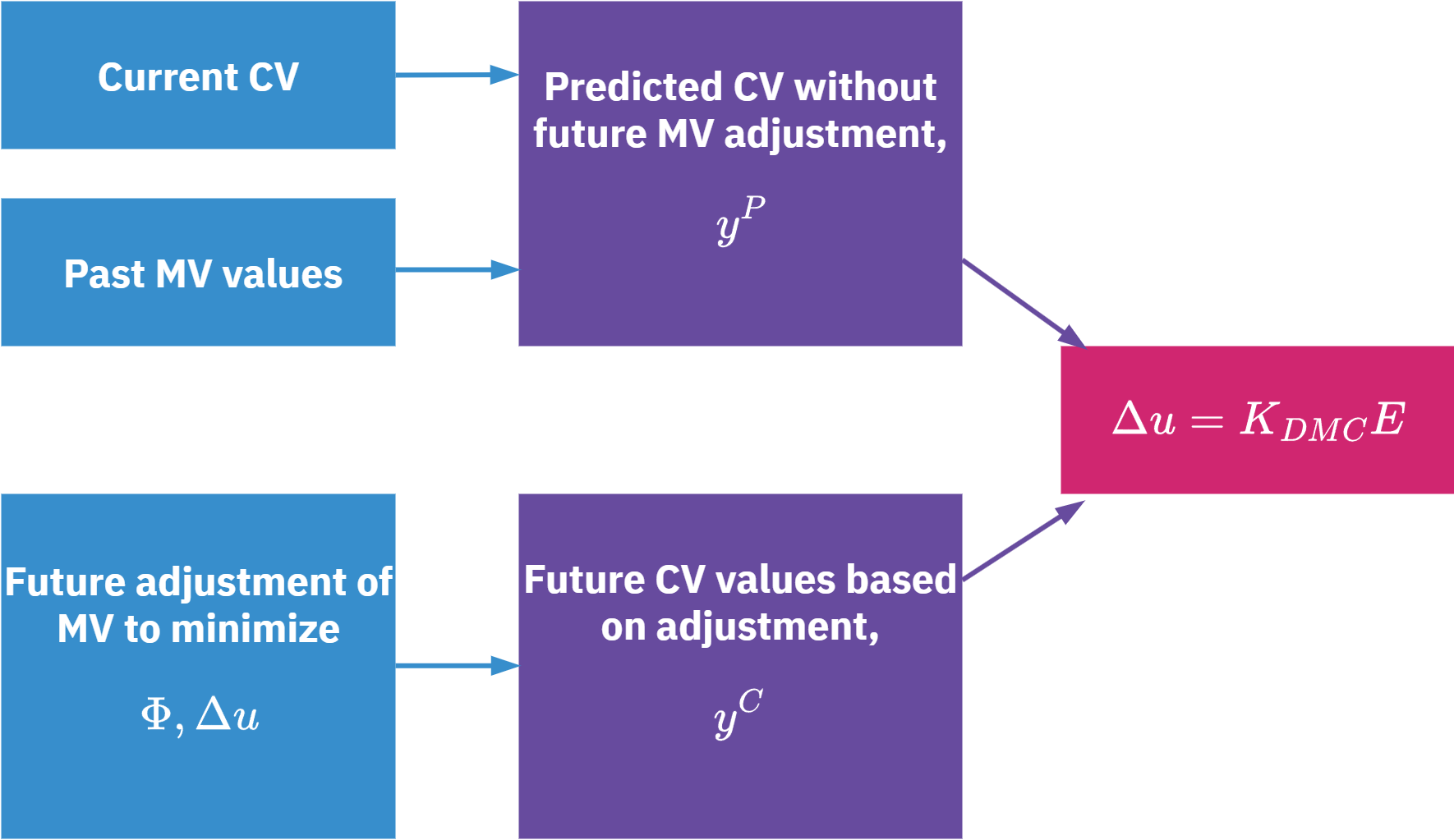
DMC Control Law

DMC control law is based on minimizing the error from setpoint $E$
The objective function $\Phi$ is the sum of the squared errors from setpoint over the prediction horizon $n$

$\Phi = \sum_{i=1}^n \bigl[y_{sp} - y(t_i)\bigr]^2$

Error term: $E(t_i) = y_{sp} - y^P(t_i) - \varepsilon$

So, $\Phi = \sum \bigl[E(t_i) - y^c(t_i)\bigr]^2$

Taking derivative: $\frac{\partial \Phi}{\partial \Delta u} = A^T \bigl(A \Delta u - E \bigr) = 0$

Hence the control law: $\Delta u = K_{DMC} E$

where $K_{DMC} = \bigl(A^T A \bigr)^{-1} A^T$

DMC computations

Move Suppression Factor Q

Basic DMC can be very aggressive
- Focuses on minimizing deviation from setpoint
- Ignores large changes in MV levels
This causes sharp changes in MV, which is undesirable
Solution: Add a move suppression term
- Introduce diagonal matrix $Q^2$ into the control law
- Penalizes rapid MV adjustments
Effect of $q$
- Larger $q$ → more penalty on $\Delta u$
- Leads to smoother, less aggressive control actions

Control law with suppression:

$\Delta u = (A^T A + Q^2)^{-1} A^T E$

Suppression matrix:

$Q = \begin{bmatrix} q & 0 & 0 & \dots & 0 \\ 0 & q & 0 & \dots & 0 \\ 0 & 0 & q & \dots & 0 \\ \vdots & \vdots & \vdots & \ddots & \vdots \\ 0 & 0 & 0 & \dots & q \end{bmatrix}$

Summary

Decouplers reduce control-loop interactions and improve performance
Two common industrial control architectures:
- Decentralized (multi-loop)
- Centralized (multivariable)
Model Predictive Control (MPC) is the most widely used multivariable controller in process industries
One of the most common MPC variants is Dynamic Matrix Control (DMC)
MPC requires a process model and an optimizer
Advantages of MPC
- Handles constraints explicitly
- Provides feedforward compensation for disturbances
- Manages process interactions effectively
- Can incorporate nonlinear models if needed
Optimal control actions are computed as

$\Delta u = K_{DMC} E$