AMC | Advanced Modeling and Control – MIMO Systems: Decentralized control

Outline

Multivariable process plants
Methods of controlling process plant
Decentralized Control vs. Centralized Control Systems
Issues in decentralized control system
Decentralized PID Control Design Methods
Decoupling controllers

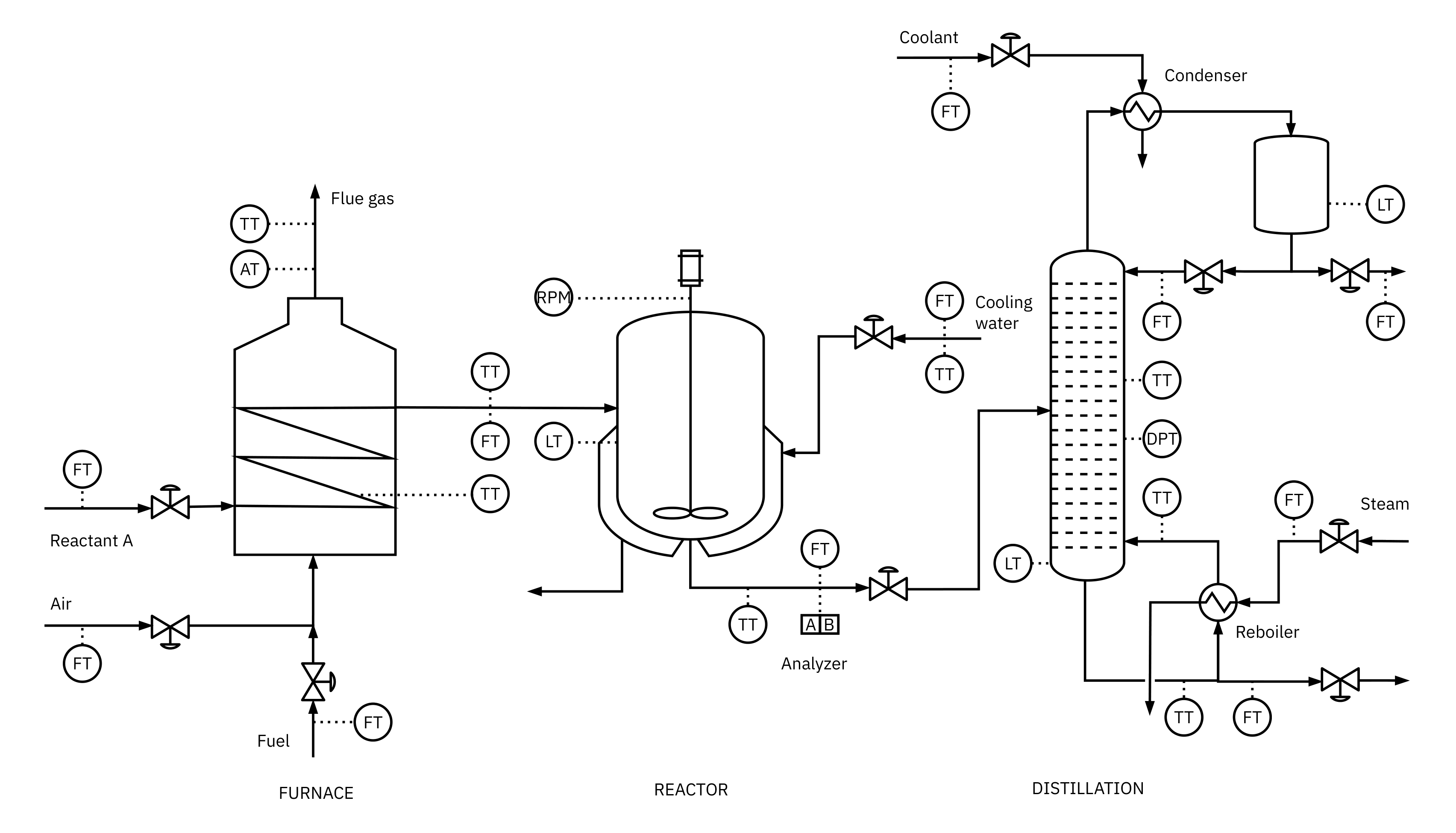
Real life processes

🤔 how many measurements are there?

Real Process often have more than one input and one outputs.
Real process has multi-input and multi-output (MIMO)
Engineers attempt to select a set of controlled variables from a set of measurement.

Plantwide control hierarchy

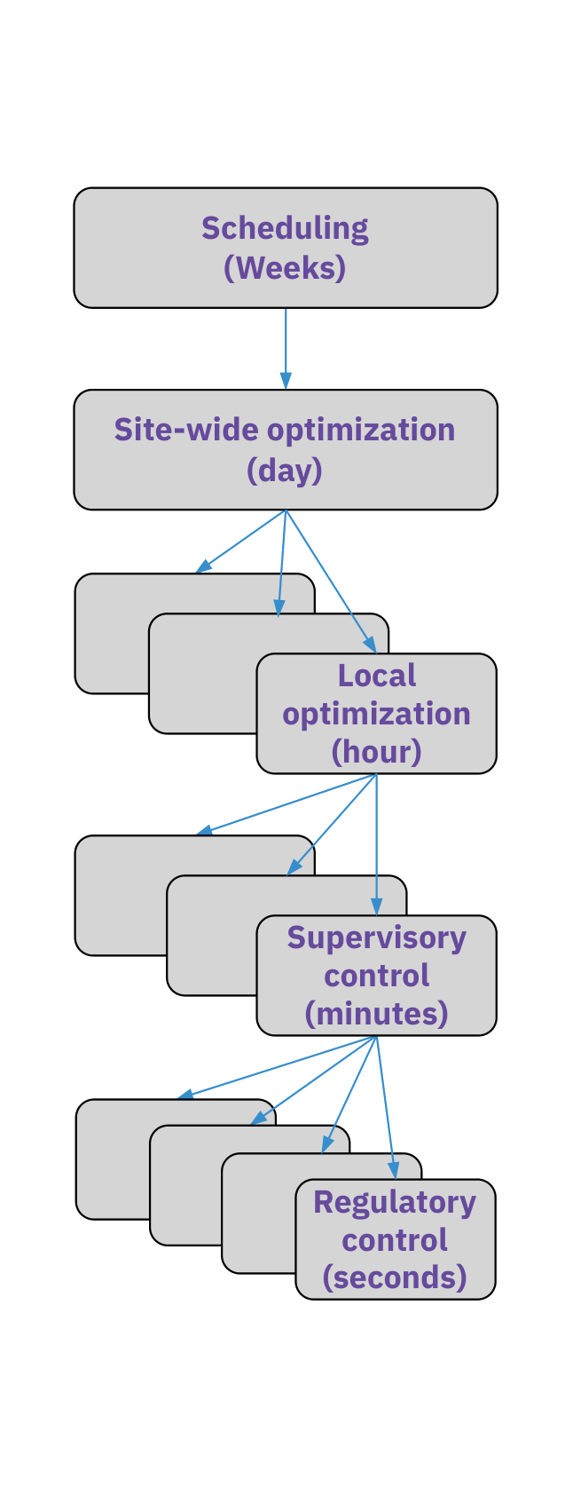
Several layers: regulatory, supervisory, optimization, scheduling.
Regulatory: multi-loop PID controls levels, temperature, flow, pressure. Ensures stability.
Supervisory: sends setpoints to the regulatory layer. May be centralized.
Optimization: real-time monitoring and optimization provide optimal targets for supervision.
Trade-off: plantwide optimization acts slower than local control.
Scheduling: inventory and production planning, often offline.

Use fast regulatory PID loops for stability, and let slower supervisory and optimization layers set plantwide targets and schedules.

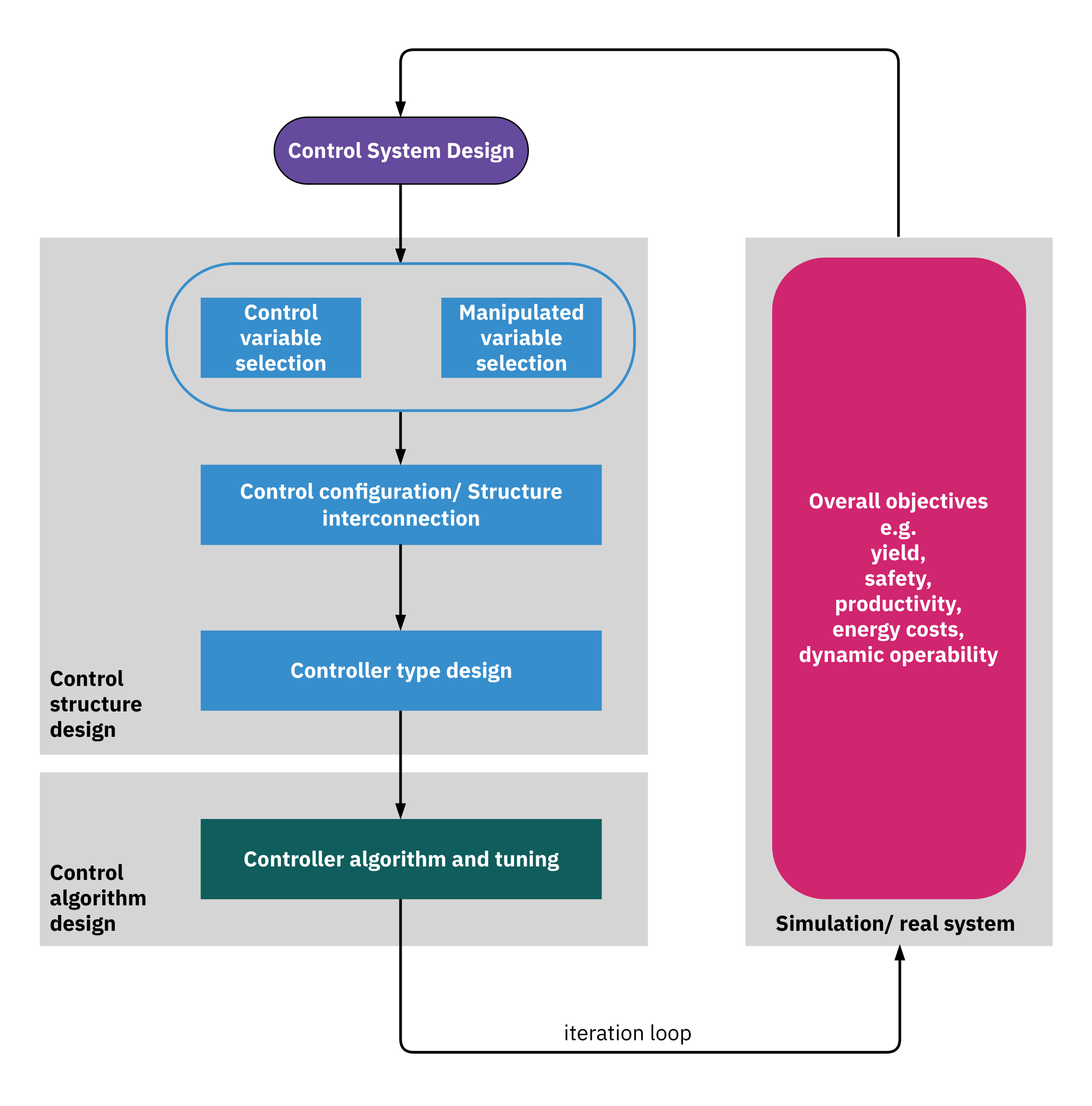
Plantwide control design flowchart

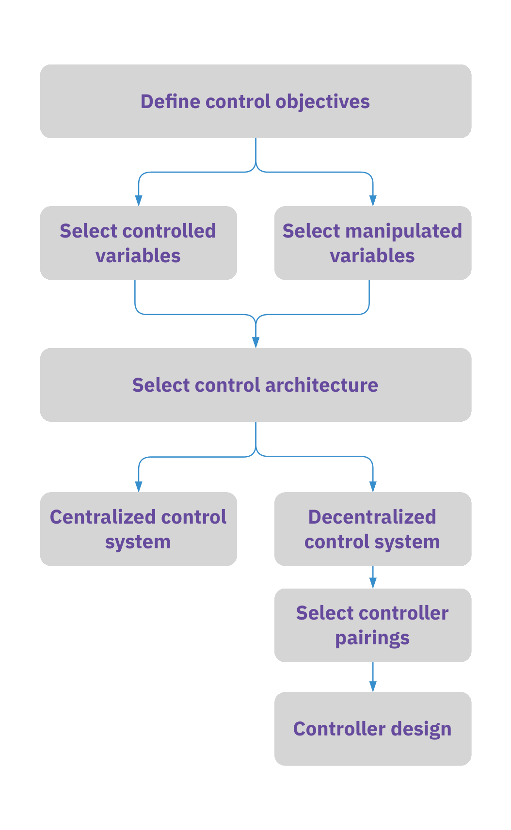
Define control objectives: explicit outcomes and implicit plantwide goals.
Select controlled and manipulated variables that support the explicit objectives and fit the plantwide philosophy.
- directly related to Explicit Control Objectives
- indirectly related to Implicit Control Objectives
Choose the control architecture: centralized or decentralized.
For decentralized (multi-loop PID) systems, decide controller pairings first to manage interactions, then design the controllers.

Plantwide control design tasks

Plantwide control design is iterative
- Choose initial controller pairings.
  
  note: different pairings may require redesign of individual controllers.
- Design and tune controllers.
- Simulate and assess plantwide performance.
  
  Use a full-plant simulation to evaluate the complete design.
- If targets are not met, revise pairings and retune.
- Repeat until objectives are satisfied.

Validate controller pairings with full-plant simulation; if KPIs fall short, revise pairings and retune until objectives are met.

Operating objectives

Purpose: Define, prioritize, and measure what “good operation” means for the unit or plant.
Priority order (use as override order)
1. Safety and compliance
2. Equipment protection and mechanical limits
3. Product quality and on-spec rate
4. Throughput and stability
5. Cost and profit
Typical objectives
- Maintain smooth operations.
- Protect equipment.
- Maximize yield of the desired product.
- Ensure safe operation.
- Minimize operating cost.
- Meet production specifications.
- Maximize profit subject to the constraints above.

Examples of control objectives

Objective	Indicator variable (unit)	Typical limit or target	Primary MV(s)	Control notes
Avoid flooding/weeping in column	Tray dP, % flood [Constraint]	dP < limit, flood < 80%	Reflux, reboiler duty, feed rate	Add dP override selectors on reflux and duty.
Protect pump (no cavitation)	NPSH margin (m) [Constraint]	Margin > required	Suction drum level, recycle valve	Use minimum flow recycle and tight level control.
Keep reactor safe	$T_{reactor}$ (°C) [CV]	< $T_{max}$ , HH trip at $T_{trip}$	Coolant flow, jacket duty	Cascade temperature to coolant valve, HH trip independent of PID.
Minimize utilities	Steam per ton, kWh per ton [Economic]	↓ vs baseline	Reboiler duty setpoint, compressor load	Supervisor trims setpoints, bounded by quality and safety.
Achieve throughput	Feed rate (t/h) [Throughput]	≥ plan	Feed valve, upstream schedule	Throughput held unless any constraint controller intervenes.

Examples of control objectives

Objective	Indicator variable (unit)	Typical limit or target	Primary MV(s)	Control notes
Avoid flooding/weeping in column	Tray dP, % flood [Constraint]	dP < limit, flood < 80%	Reflux, reboiler duty, feed rate	Add dP override selectors on reflux and duty.
Protect pump (no cavitation)	NPSH margin (m) [Constraint]	Margin > required	Suction drum level, recycle valve	Use minimum flow recycle and tight level control.
Keep reactor safe	$T_{reactor}$ (°C) [CV]	< $T_{max}$ , HH trip at $T_{trip}$	Coolant flow, jacket duty	Cascade temperature to coolant valve, HH trip independent of PID.
Minimize utilities	Steam per ton, kWh per ton [Economic]	↓ vs baseline	Reboiler duty setpoint, compressor load	Supervisor trims setpoints, bounded by quality and safety.
Achieve throughput	Feed rate (t/h) [Throughput]	≥ plan	Feed valve, upstream schedule	Throughput held unless any constraint controller intervenes.

Mapping objectives to CVs and MVs

Pick CVs and MVs that directly support each objective.
Put constraint controllers in place first (safety, equipment limits, environmental).
Add quality and inventory loops next, then throughput, then cost optimization.
Use override selectors so higher-priority loops take control when limits approach.
Provide simulation or digital twin checks for KPI impact before moving setpoints.
Document alarms and trips (setpoint, alarm, trip) for each safety-critical KPI.

Control strategy must achieve the entire set of objectives

2x2 MIMO process system

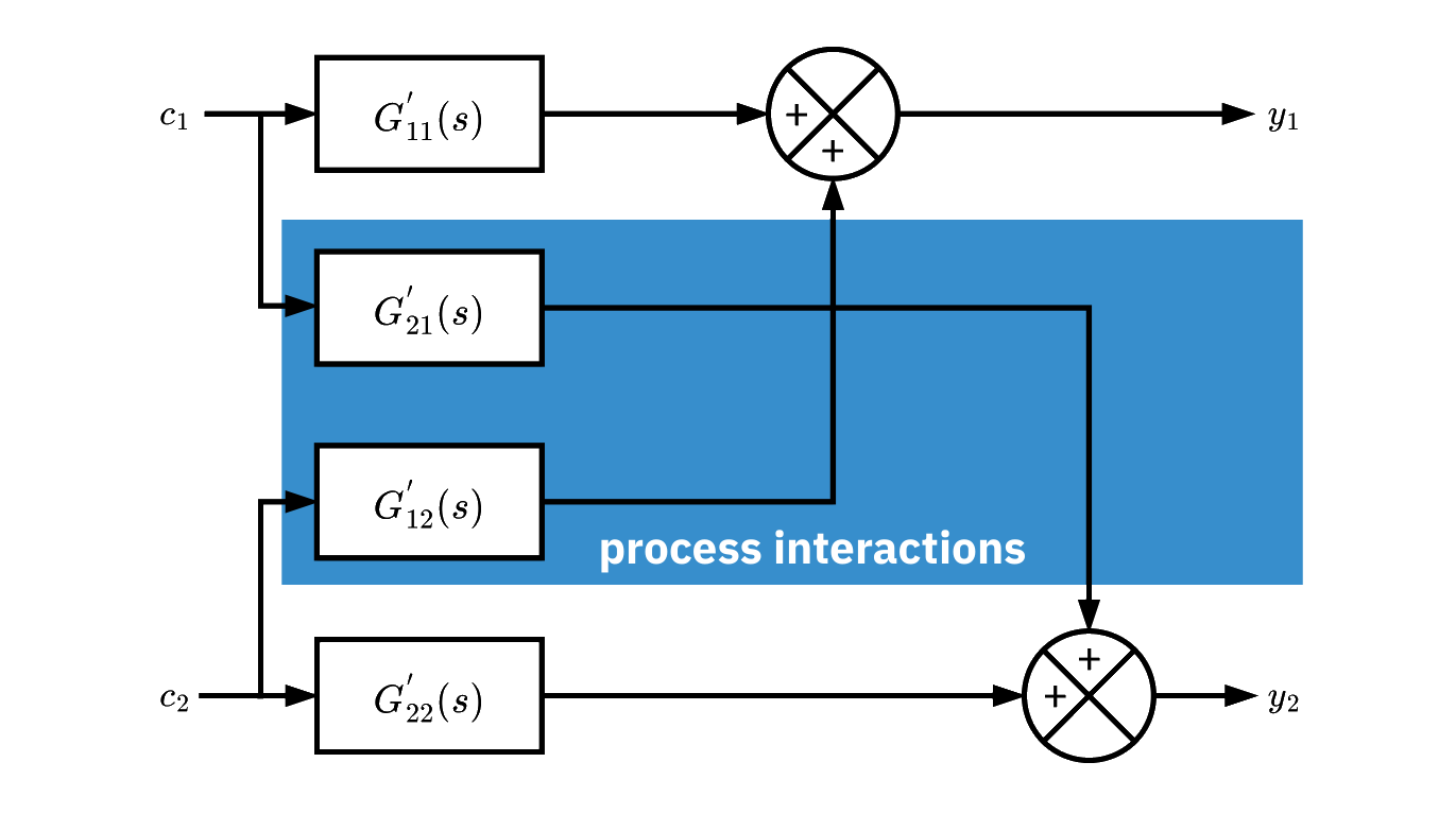
Inputs: $c_1, c_2$ . Outputs: $y_1, y_2$ .
Plant ransfer function matrix
$\mathbf{G}=\begin{bmatrix} G'_{11} & G'_{12} \\ G'_{21} & G'_{22} \end{bmatrix}$
$G'_{12}$ is the transfer from $c_2$ to $y_1$ .
Interactions: a change in $c_1$ or $c_2$ affects both outputs.
Cross terms $G'_{12}$ and $G'_{21}$ create loop coupling.
Interactions can limit decentralized control performance.

Distillation column: 2x2 MIMO example

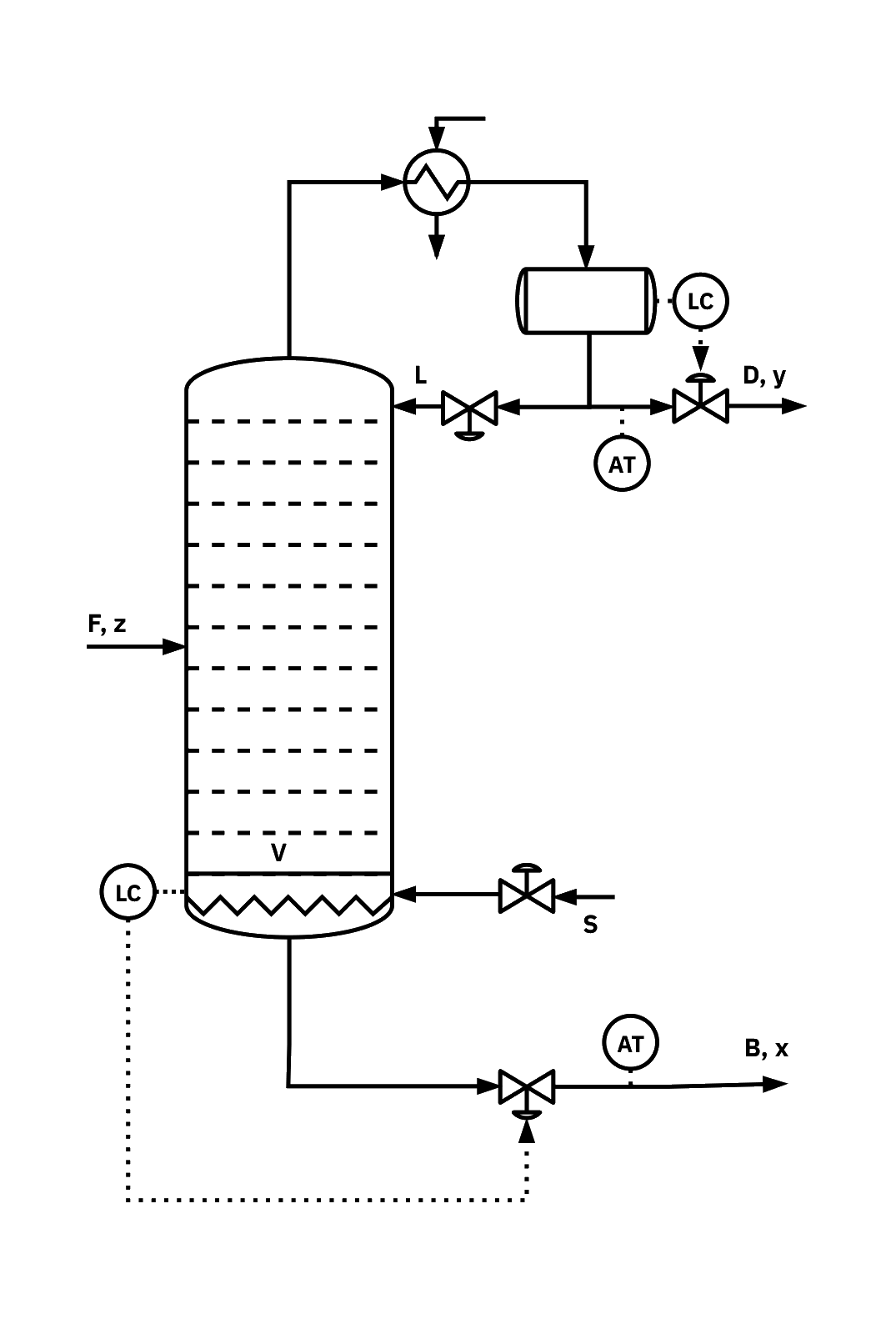
Two inputs: reflux flow $L$ , steam/boilup $S$ .
Two outputs: distillate composition $y_D$ , bottoms composition $x_B$ .
Interactions: changes in $L$ or $S$ affect both $y_D$ and $x_B$ .
Level loop: weakly coupled to compositions.
Design focus: composition controllers; choose pairings/decoupling to handle interactions.

Controller pairings

One major task in decentralized control system design → to select controller pairings
Controller pairings are chosen based on 3 main factors:
1. Process Interactions
2. Dynamic responses
3. Sensitivity to disturbances
Improper controller pairings can lead to severe process interaction → causes poor control performance
Factors can be conflicting with each other
- e.g., pairings that lead to minimum process interactions may exhibit slow dynamic responses
- it is desirable to have fast dynamic responses.

multi‐loop controllers (decentralized)

Two SISO loops, two controllers.
Independence is only valid when interactions are negligible.
Cross terms $G'_{21}$ and $G'_{12}$ couple the loops and affect tuning.
Direct pairings: $c_1 \rightarrow y_1$ , $c_2 \rightarrow y_2$ .
Indirect pairings: $c_1 \rightarrow y_2$ , $c_2 \rightarrow y_1$ .
Pairing choice changes interaction severity and overall performance.

Multi‐loop controllers – distillation column

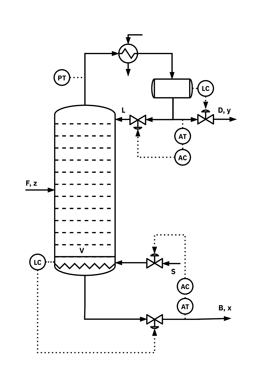
Reflux flow $L$ controls top composition $y_D$ .
Steam/boilup $S$ controls bottom composition $x_B$ .
Bottoms flow $B$ maintains level.
Top and bottom composition loops are strongly coupled, level loop coupling is weak.
Select composition pairings to manage interactions. Compare $L\!\to\!y_D$ , $S\!\to\!x_B$ with the swapped pairing using gains, dynamics, and disturbance paths.

🤔

Can we control the top composition using the steam flow, while the bottom composition using the reflux flow? Why ?

Usually no for decentralized PID.

Prefer reflux → top composition and steam/boilup → bottom composition.

Why?

Sensitivity: typically $|\partial y_D/\partial L| \gg |\partial y_D/\partial S|$ and $|\partial x_B/\partial S| \gg |\partial x_B/\partial L|$ . The RGA diagonal for the direct pairing is positive and near 1, while the swapped pairing gives small or even negative diagonals, meaning strong interaction.
Dynamics: $L \to y_D$ and $S \to x_B$ are faster, with shorter delays. The cross paths $S \to y_D$ and $L \to x_B$ are slower and can show inverse or sluggish response, so the loops fight.
Disturbance rejection: common disturbances (feed rate, composition) are rejected more effectively with the direct pairing; the swapped pairing corrects via long, weak paths and tends to oscillate or saturate.

Exception

If your operating point gives RGA diagonals for the swapped pairing that are positive and close to 1, and step tests show comparable or faster dynamics, it can work. Otherwise, stick to the standard pairing or use multivariable control with decoupling.

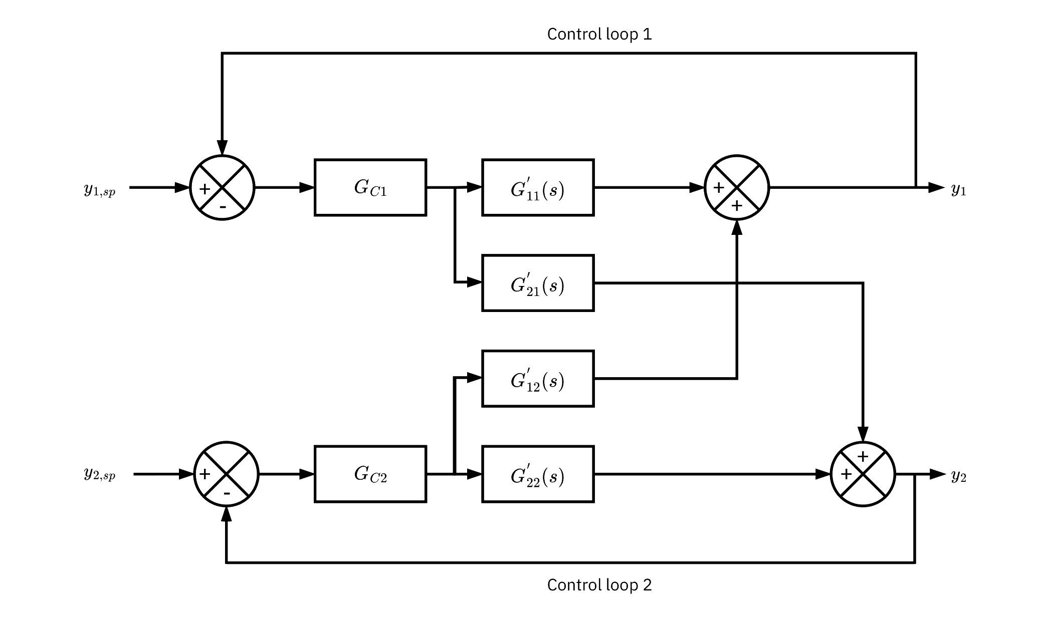
Coupling effect of loop 2 on $y_1$

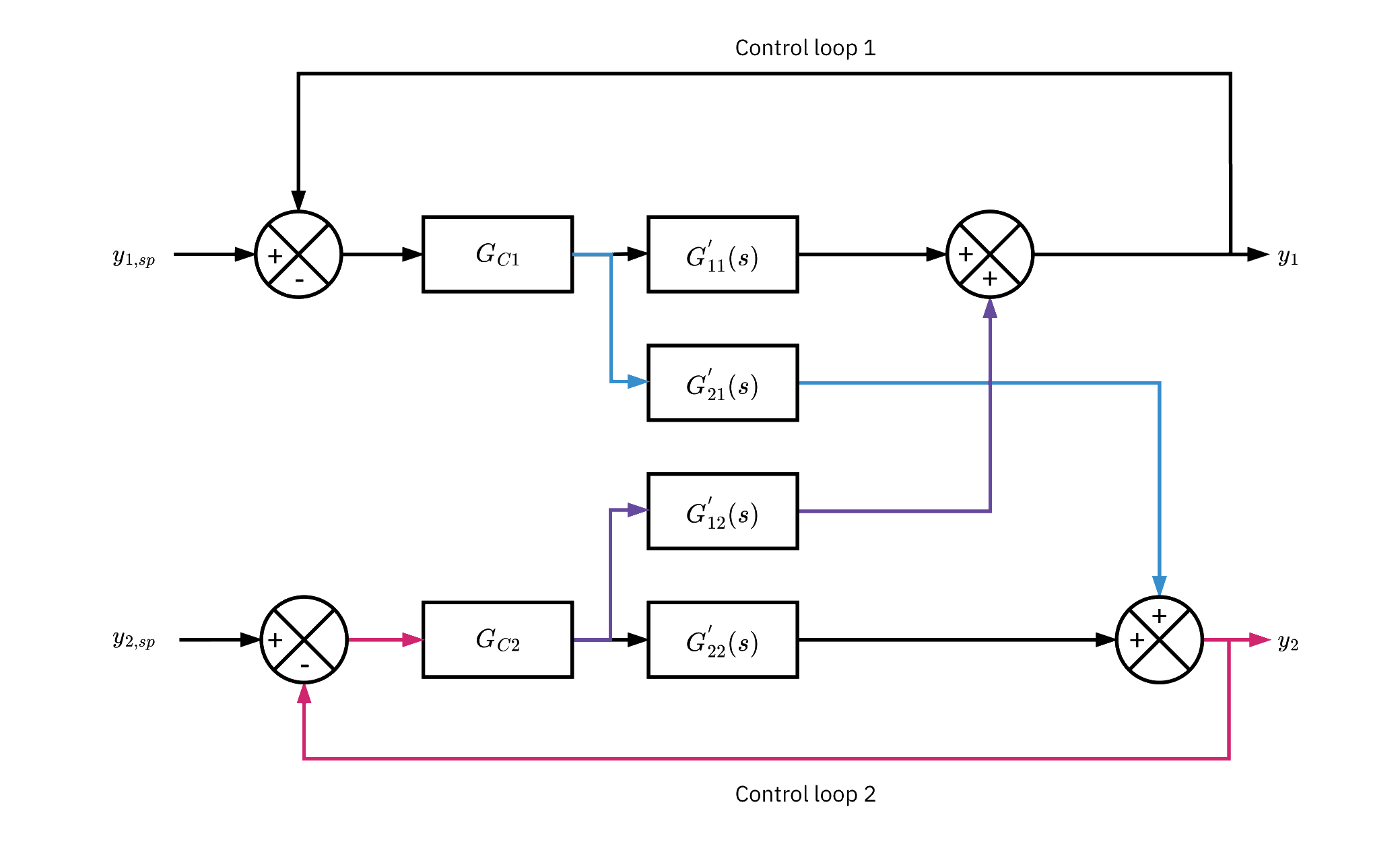
Change $y_{1,\mathrm{sp}}$ → controller $G_{C1}$ moves $c_1$ .
$c_1$ impacts $y_1$ via $G'_{11}$ and $y_2$ via $G'_{21}$ .
$y_2$ deviates → $G_{C2}$ adjusts $c_2$ .
$c_2$ impacts $y_2$ via $G'_{22}$ and $y_1$ via $G'_{12}$ .
Loop 1 reacts again to the cross effect on $y_1$ .
The loops iterate until $y_1$ and $y_2$ settle, if no further setpoint or disturbance changes occur.

Multi‐loop controllers – distillation column

Reflux $L$ holds the distillate composition $y_D$ ; changing $L$ also disturbs the bottoms composition $x_B$ .
The bottoms loop reacts: adjust steam/boilup $S$ to bring $x_B$ back to its setpoint.
That change in $S$ disturbs $y_D$ ; the reflux loop trims $L$ until $y_D$ returns to setpoint.

Relative Gain Array - steady-state interaction

Relative Gain Array (RGA) is a steady-state interaction measure for MIMO systems.

$\Lambda=K\circ (K^{-1})^{\mathsf T}$

$K$ is the steady-state gain matrix of linearized plant. Its entries are the open-loop gains
$K^{-1}$ is the inverse of $K$
$(\cdot)^{\mathsf T}$ is transpose,
$\circ$ is the Hadamard (element-wise) product.
The RGA element is thus $\lambda_{ij}=k_{ij}\,(K^{-1})_{ji}.$

For a 2×2 system

$\Lambda =\begin{bmatrix}\lambda_{11}&\lambda_{12}\\\lambda_{21}&\lambda_{22}\end{bmatrix}$

$\lambda_{11}=\lambda_{22}=1-\frac{k_{12}k_{21}}{k_{11}k_{22}}$ $\lambda_{12}=\lambda_{21}=\frac{k_{12}k_{21}}{k_{11}k_{22}}$

Properties
Row and column sums: $\sum_j \lambda_{ij}=1 \qquad \sum_i \lambda_{ij}=1$
For 2×2, the diagonal terms are equal: $\lambda_{11}=\lambda_{22}; \quad \lambda_{11}+\lambda_{12} = 1; \quad \lambda_{21}+\lambda_{22} = 1$

Relative Gain Array - steady-state interaction

For 2×2, only one element requires evaluation: $\lambda_{11} = \frac{ \overbrace{ \left(\dfrac{\Delta y_{1}}{\Delta c_{1}}\right)_{c_{2}} } ^{ {\color{#9f1853} \text{main effect (}2^{\text{nd}}\text{ loop open)} } } }{ \underbrace{ \left(\dfrac{\Delta y_{1}}{\Delta c_{1}}\right)_{y_{2}} }_{ {\color{#9f1853} \text{main + coupling (}2^{\text{nd}}\text{ loop closed)} } } }$

RGA for higher-order MIMO (3×3, 4×4)
- Definition stays the same: $\Lambda = K \circ (K^{-1})^{\mathsf T}$
- Key properties for $n\times n$ :
- Row sums and column sums equal 1.
- Diagonals need not be equal and $\Lambda$ need not be symmetric.
- Scale invariant, but operating-point dependent.

RGA does not change if you rescale variables or change units
RGA needs to be recomputed when the operating point shifts

RGA: coupling effect (interpretation of $\lambda_{11}$ )

$\lambda_{11}=1$ — no coupling.
$0<\lambda_{11}<1$ — coupling in the same direction as the main effect; severity grows as $\lambda_{11}\!\downarrow$ .
At $\lambda_{11}=0.5$ : very severe.
$\lambda_{11}>1$ — coupling in the opposite direction; severity grows as $\lambda_{11}\!\uparrow$ .
$\lambda_{11}<0$ — sign reversal / very strong coupling; risk of closed-loop instability → avoid that pairing.
Choosing pairings for $n\times n$ :
- Select one element per row and column (a permutation) with positive $\lambda_{ij}$ near 1.
- Practical rule: minimize cost matrix $C_{ij}=|\lambda_{ij}-1|$ with an assignment method (for example Hungarian), or use a greedy pick (per row choose the available column with the smallest $C_{ij}$ and $\lambda_{ij}>0$ ).

Negative or near-zero $\lambda_{ij}$ indicates problematic pairings.
Many large off-diagonals in a row or column imply strong interaction → consider decoupling or multivariable control.

RGA calculation

Given a $2\times2$ transfer-function matrix (FOPTD elements):

$G(s)= \begin{bmatrix} \dfrac{k_{11}e^{-\theta_{11}s}}{\tau_{11}s+1} & \dfrac{k_{12}e^{-\theta_{12}s}}{\tau_{12}s+1} \\[6pt] \dfrac{k_{21}e^{-\theta_{21}s}}{\tau_{21}s+1} & \dfrac{k_{22}e^{-\theta_{22}s}}{\tau_{22}s+1} \end{bmatrix}$
Steady-state gain matrix:

$K=\begin{bmatrix}k_{11}&k_{12}\\k_{21}&k_{22}\end{bmatrix}$
Relative Gain Array:

$\Lambda=K\circ (K^{-1})^{\mathsf T} =\begin{bmatrix}\lambda_{11}&\lambda_{12}\\\lambda_{21}&\lambda_{22}\end{bmatrix}$

Diagonal element:

$\lambda_{11} =\frac{k_{11}}{\underbrace{k_{11}}_{\text{main}}-\underbrace{\dfrac{k_{12}k_{21}}{k_{22}}}_{\text{coupling}}} =\frac{1}{1-\dfrac{k_{12}k_{21}}{k_{11}k_{22}}}$

MATLAB:

Lambda = K .* (inv(K)).';
% numerically safer but computationally expensive
% Lambda = K .* (pinv(K)).';

Activity 4 (i, ii, iii): Steady-state RGA

RGA analysis

Good for: assessing the steady-state coupling effect of a configuration.
Applicable when input/output relationships have the same general dynamic behaviors.
Pairing rules
- Prefer $\lambda_{ij}$ closest to 1 (weakest interaction).
- Avoid $\lambda_{ij}\le 0$ (sign reversal / integrity risk—one loop failure can destabilize the other).
- Ensure a one-to-one mapping (one element per row and column).
Caution: can be misleading if transfer-function dynamics are significantly different.
Bottom line: RGA is a steady-state measure of process interaction.

Impact of dynamic behavior

Process Transfer Functions

$G_{11}(s) = \frac{1.0}{100s+1}, \quad G_{12}(s) = \frac{0.3}{10s+1}$

$G_{21}(s) = \frac{-0.4}{10s+1}, \quad G_{22}(s) = \frac{2.0}{100s+1}$

Steady-State Gain Matrix

$K = \begin{bmatrix} 1.0 & 0.3 \\ -0.4 & 2.0 \end{bmatrix}$

Relative Gain Array (RGA)

$\lambda_{11} = \frac{1}{1 - \frac{K_{12}K_{21}}{K_{11}K_{22}}} = \frac{1}{1 - \frac{(0.3)(-0.4)}{(1.0)(2.0)}} = 0.94$

$\Lambda = \begin{bmatrix} 0.94 & 0.06 \\ 0.06 & 0.94 \end{bmatrix}$

Impact of dynamic behavior

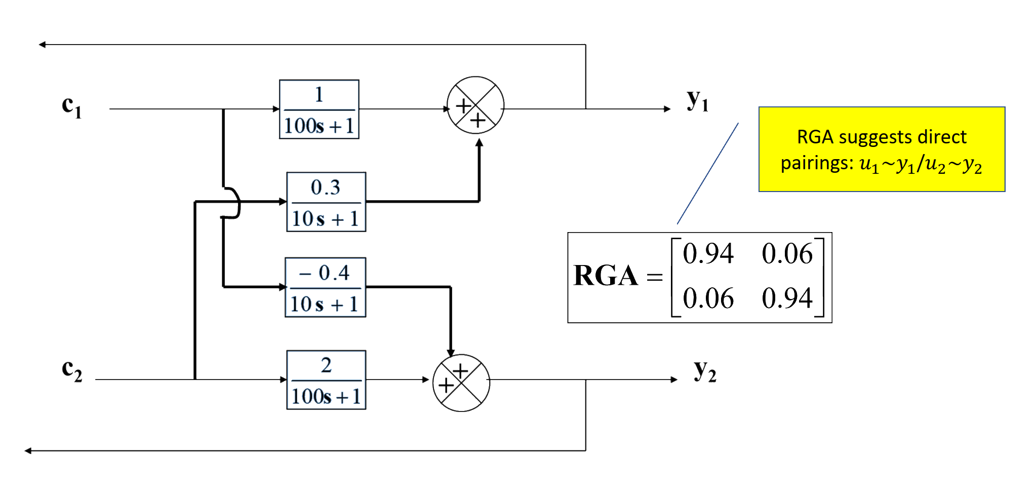
Direct vs reverse pairing

RGA suggests direct pairings: $u_1 \to y_1$ , $u_2 \to y_2$ .
But time-domain simulations show reverse pairings outperform direct pairings.
Dynamic responses of two transfer functions differ (time constants 100 s vs 10 s).
Steady-state RGA alone may be misleading; dynamic RGA is needed.

Dynamic RGA

When transfer function dynamics differ significantly, steady-state RGA can be misleading.
Dynamic RGA evaluates interaction strength as a function of frequency ω.
Helps identify correct pairings depending on operating frequency range.

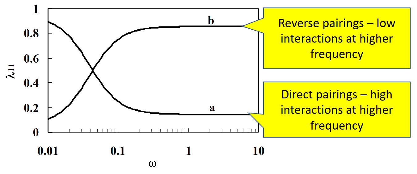
Mathematical Formulation

$\lambda_{11}(\omega) = \frac{1}{ 1 - \frac{|G_{12}(i\omega)||G_{21}(i\omega)|}{|G_{11}(i\omega)||G_{22}(i\omega)|} }$

For a first-order process:

$|G(i\omega)| = \frac{K_p}{\sqrt{\tau_p^2 \omega^2 + 1}}$

For the example system:

$\lambda_{11}(\omega) = \frac{1}{1 + \frac{16.7(100^2\omega^2 + 1)}{100^2\omega^2 + 1}}$

Pairing Considerations

Choose pairing between manipulated and controlled variables that results in the least process interactions.
- Use steady-state RGA for comparable dynamics.
- Use dynamic RGA for dissimilar dynamics.
Choose pairing that leads to quick response of controlled variable to manipulated variable (fast dynamic criterion).
- Example:
  
  $\frac{Y_1}{U_1} = \frac{2 e^{-s}}{10s+1}, \quad \frac{Y_1}{U_2} = \frac{2 e^{-3s}}{12s+1}$
  
  Prefer $U_1 \sim Y_1$ because $U_1$ responds faster. $U_2$ has longer deadtime, which reduces achievable control performance.
Choose pairing that is least sensitive to disturbance.
Key Insights
- Direct pairings can suffer at higher frequency if dynamics are mismatched.
- Reverse pairings may be more effective at higher frequency, even if steady-state RGA suggests otherwise.
- Rule of thumb:
  - Low frequency operation → direct pairings
  - High frequency operation → reverse pairings

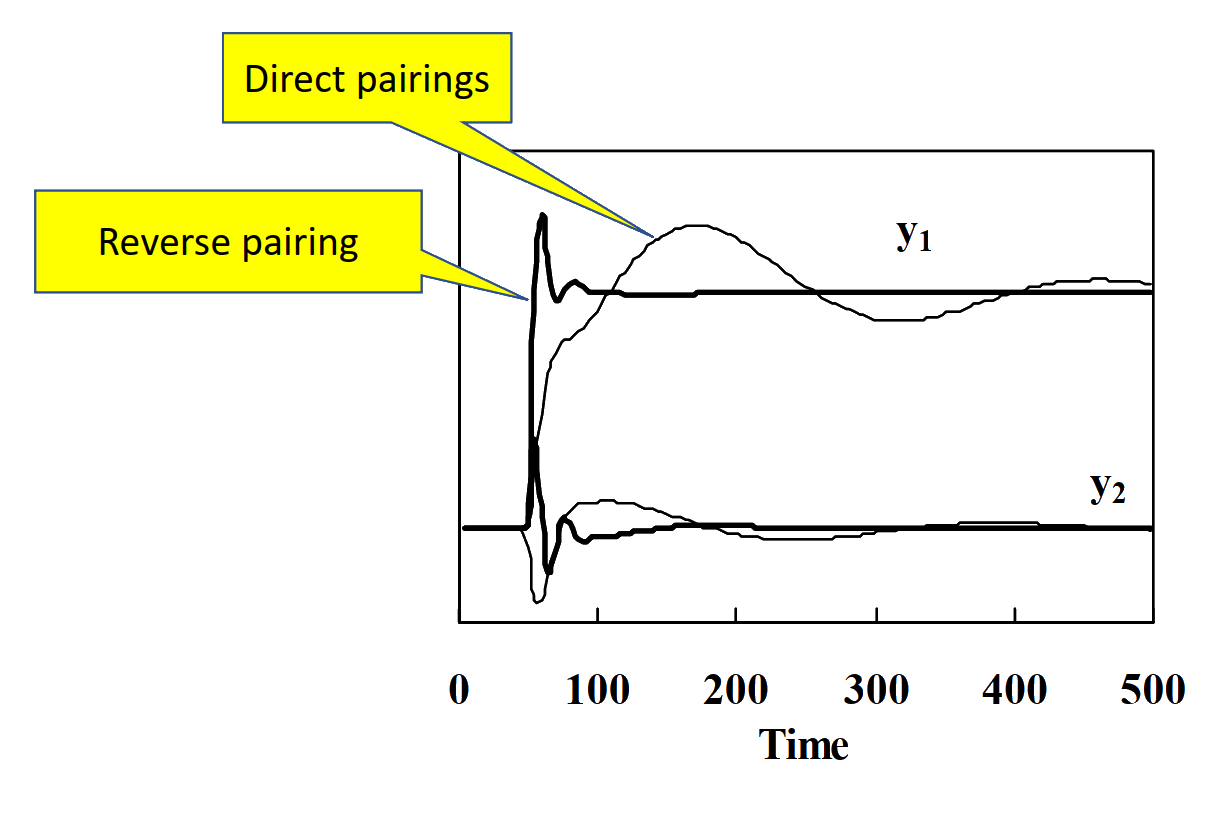
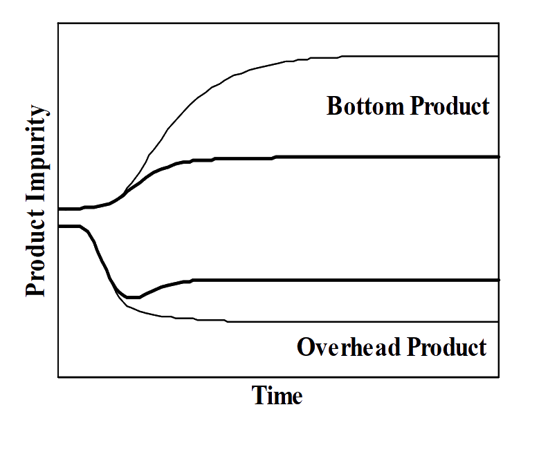
Sensitivity to disturbances

Each configuration has a different sensitivity to a disturbance.
Thick and thin line represent the results of different configurations.
Notice that, the configuration with thick line is less sensitive to disturbance than the one with thin line.
The one that is less sensitive to disturbance is a more efficient configuration (or pairings).
Less sensitive to disturbance is also good because it could lead to lower control action required.

Example ‐ configuration selection for a C3 splitter

Configuration	RGA (λ₁₁)	Comment
(L, B)	0.94	Least interactions
(L, V)	25.3	Severe interactions – coupling effect opposite to main effect
(L/D, V/B)	1.70	Mild interactions
(D, V)	0.06	Mild interactions – coupling effect in same direction as main effect; main effect weaker than coupling effect

(L,V) configuration applied to the C3 splitter

Reflux flow $L$ is used to control top composition
Steam flow $S$ is used to control bottom composition
Steam flow directly affects vapor flow $V$ in the column → therefore $V$ is used to control the bottom composition
This arrangement is known as the (L,V) configuration

Reflux ratio applied to the overhead of the C3 splitter

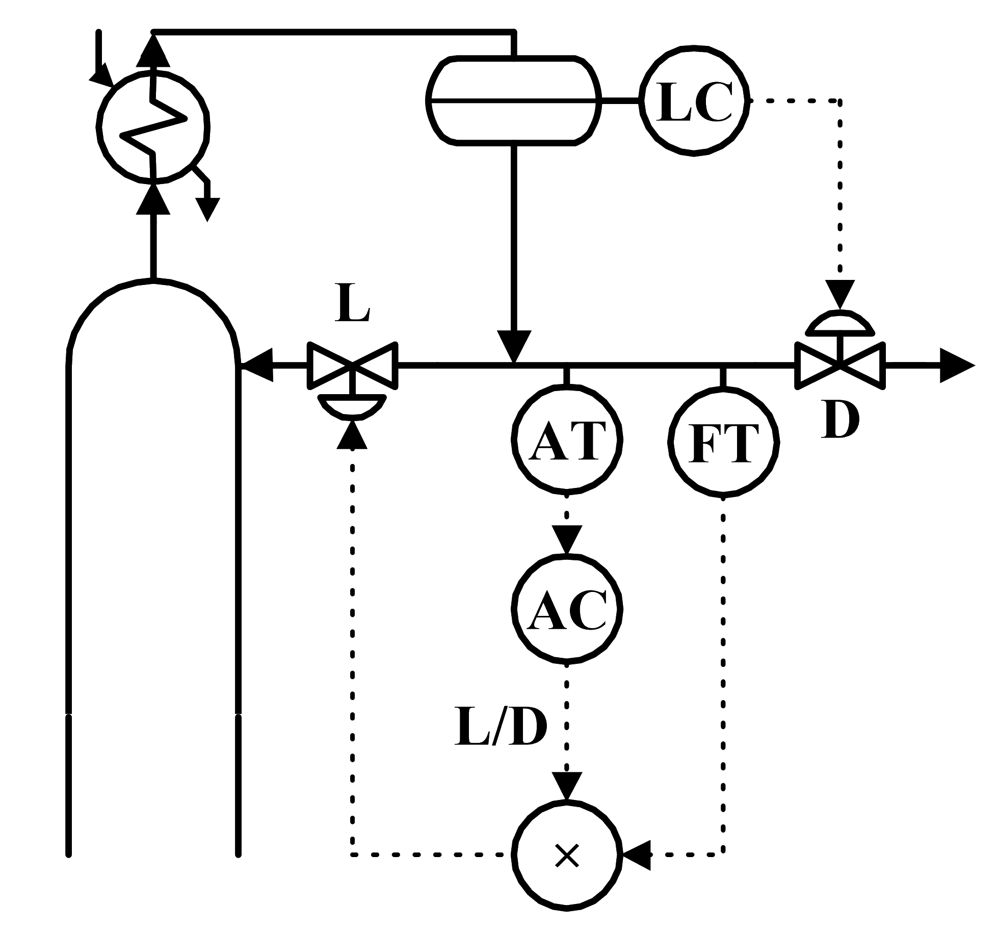
Ratio controller is used where the wild stream is the distillate flow, while the reflux stream is the manipulated flow
Thus, reflux ratio (L/D) is used as manipulated variable by the top composition controller
For the bottom composition controller, the boilup ratio (V/B) can be used as manipulated variable
- Bottom flow B is wild stream
- Steam flow S is the manipulated stream (S is directly related to vapor flow
Thus, this is called the (L/D, V/B) configuration

Other configurations

(L,B) configuration
- Reflux flow L is used to control top composition
- Bottom flow B is used to control bottom composition
(D,V) configuration
- Distillate flow D is used to control top composition
- Steam flow (related directly to V) is used to control bottom composition

Configuration selection of C3 splitter

L, L/D and V are the least sensitive to feed composition disturbances
L and V have the most immediate effect on the product compositions
L/D and V/B give an intermediate effect
D and B yield the slowest response
Each configuration involves conflicting factors
- Example: (L,V) is the least sensitive to disturbance and has fast dynamic response
- But it exhibits the most severe process interaction (λ11 = 25.3)
Therefore, simulation is required to evaluate configuration performance

Control performance

Configuration	IAE for Overhead	IAE for Bottoms
(L, B)	0.067	1.49
(L, V)	0.250	13.3
(L/D, V/B)	0.095	2.00
(D, V)	0.098	1.91

(L,B) configuration gives the smallest IAE for the overhead controller
Indicates best top controller performance
Also corresponds to the configuration with least interactions

Analysis of configuration selection example

(L,V) is the worst configuration
- It is the least susceptible to disturbances and the fastest acting configuration
- But it is the most coupled (λ11 = 25.3)
(D,V) has an RGA of 0.06 but shows decent control performance
- D has slow dynamic, V has fast dynamic
- If both had fast or both had slow dynamics, this configuration might show poor performance
(L,B) is the best configuration
- Provides good decoupling
- Overhead product is most important

Multi‐loop (decentralized) pid controller design

There are six main categories of methods to design multi-loop PID control systems:

Detuning
Sequential loop closing
Independent tuning
Simultaneous tuning
Optimization
Relay auto-tuning

Key Idea

Each method offers a different balance of: - Simplicity vs. performance
- Handling of interactions
- Practical implementation effort

Detuning method

Step 1: An individual controller is tuned according to an existing single-input and single-output tuning formula, e.g., classical Ziegler-Nichols and Skogestad IMC
- Example: consider 2 multi-loop PID controllers
  $G_{c1} = K_{c1} \left( 1 + \frac{1}{\tau_{I1} s} + \tau_{D1} s \right), \quad G_{c2} = K_{c2} \left( 1 + \frac{1}{\tau_{I2} s} + \tau_{D2} s \right)$
Step 2: Detune each controller by a factor F
- Detuned controllers
  $G'_{c1} = \frac{K_{c1}}{F} \left( 1 + \frac{1}{\tau_{I1} s} + \tau_{D1} s \right), \quad G'_{c2} = \frac{K_{c2}}{F} \left( 1 + \frac{1}{\tau_{I2} s} + \tau_{D2} s \right)$
Step 3: Evaluate the closed-loop responses – if not satisfied then readjust F

Example 2x2 MIMO – Wood and Berry (WB) column

The Wood and Berry column is represented by the transfer function matrix

$G = \begin{bmatrix} \frac{12.8 e^{-s}}{16.7s + 1} & \frac{-18.9 e^{-3s}}{21s + 1} \\ \frac{6.6 e^{-7s}}{10.9s + 1} & \frac{-19.4 e^{-3s}}{14.4s + 1} \end{bmatrix}$

RGA analysis

$\Lambda = \begin{bmatrix} 2.0094 & -1.0094 \\ -1.0094 & 2.0094 \end{bmatrix}$

Recommended pairings: $U_1 \rightarrow Y_1$ and $U_2 \rightarrow Y_2$ (direct pairings)
Direct pairings ensure RGA elements are positive
Always avoid negative RGA pairings

WB column - detuning method

Apply Ziegler-Nichols tuning (Matlab Control System Designer) to design two PID controllers
Design PID 1 based on
$g_{11} = \frac{12.8 e^{-s}}{16.7s+1}$
$G_{c1} = 1.2895 \left( 1 + \frac{1}{2s} + 0.4602s \right), \quad GM = 5.02 \, dB, \, PM = 34.9^\circ$
Design PID 2 based on
$g_{22} = \frac{-19.4 e^{-3s}}{14.4s+1}$
$G_{c2} = -0.2548 \left( 1 + \frac{1}{5.6s} + 1.4s \right), \quad GM = 4.88 \, dB, \, PM = 40.1^\circ$

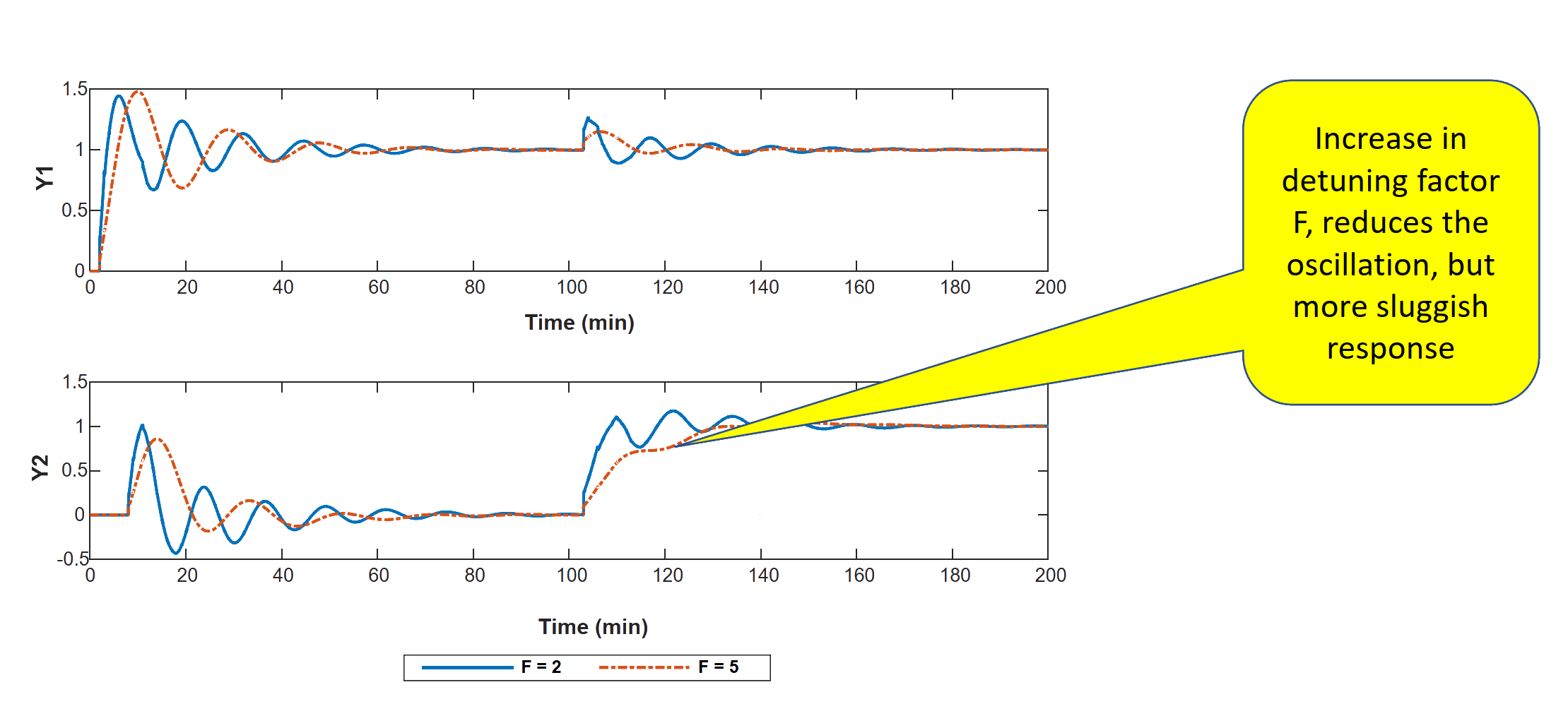
WB column - detuning method

If F = 2
$G'_{c1} = 0.6448 \left( 1 + \frac{1}{2s} + 0.4602s \right), \quad G'_{c2} = -0.1274 \left( 1 + \frac{1}{5.6s} + 1.4s \right)$
If F = 5
$G'_{c1} = 0.2579 \left( 1 + \frac{1}{2s} + 0.4602s \right), \quad G'_{c2} = -0.0510 \left( 1 + \frac{1}{5.6s} + 1.4s \right)$

Sequential loop (SQL) closing

Steps
1. Choose the fast loop first, before the slower one
2. Design the controller for the faster loop using its transfer function
3. Close the fast loop (activate controller)
4. Derive a linearized model for the slower loop with the fast loop already closed
5. Design the second controller using the linearized model
6. Close the second (slower) loop
For additional loops, repeat steps 4 to 6

The order of loop closing is critical as it strongly influences overall control performance

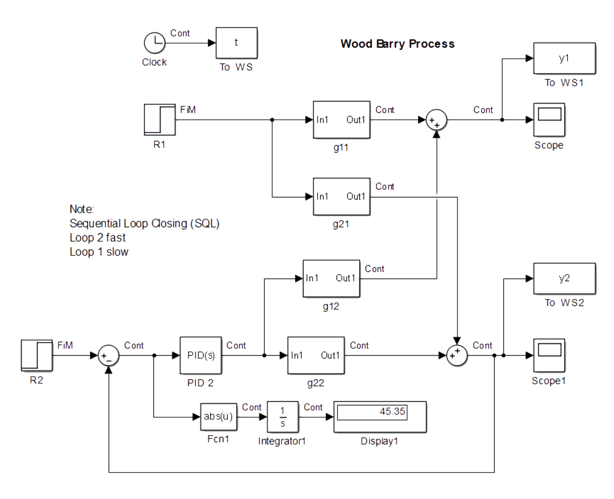
WB column – SQL method

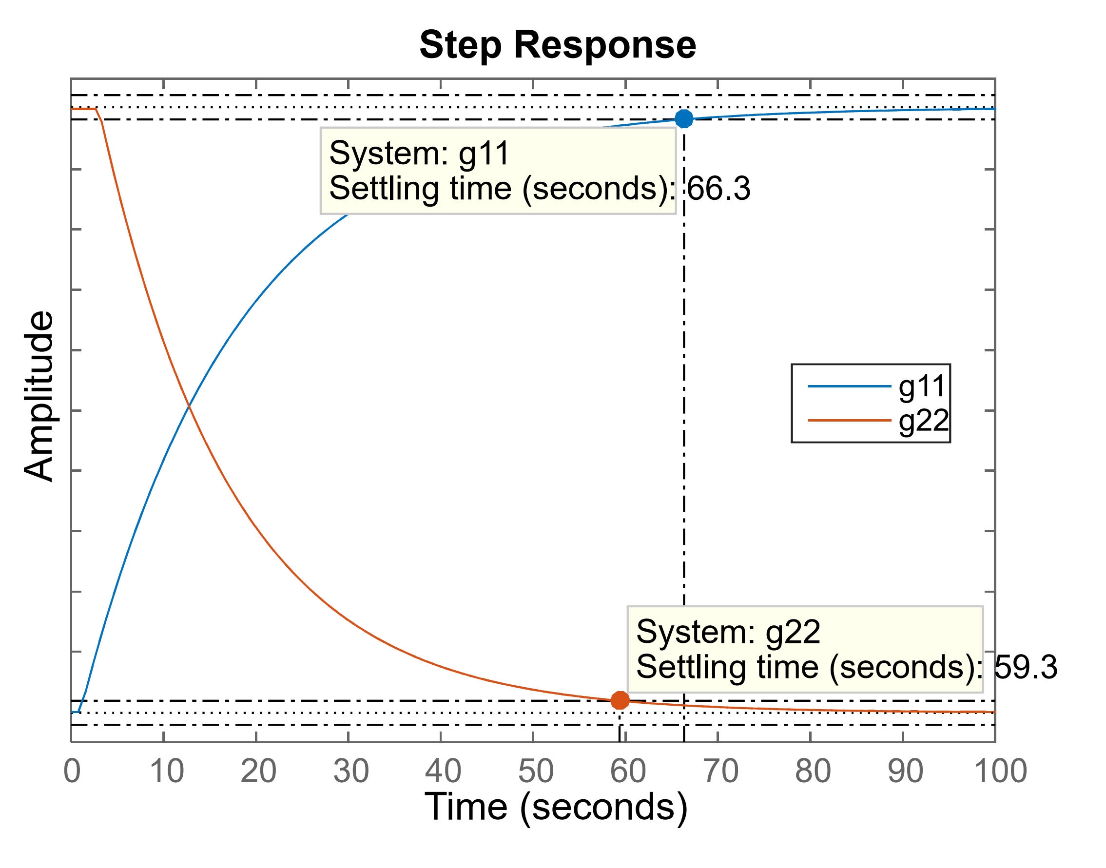
Step 1: Identify which loop is faster by comparing open-loop step responses of $g_{11}$ and $g_{22}$
Use Matlab commands:

  s = tf('s');
  g11 = 12.8*exp(-s)/(16.7*s + 1);
  g22 = -19.4*exp(-3*s)/(14.4*s + 1);
  step(g11, g22);

From the step responses:
- $g_{22}$ has a shorter settling time (59.3 s)
- $g_{11}$ has a longer settling time (66.3 s)
- Therefore, loop 2 is faster than loop 1

Sequential loop closing example

use skogestad imc (simc) tuning in matlab control system designer
design pid 2 using $g_{22}$

$g_{c2} = -0.1423 \left( 1 + \frac{1}{16.5s} + 1.3636s \right)$

$gm = 9.71 \, db, \quad pm = 74.8^\circ$
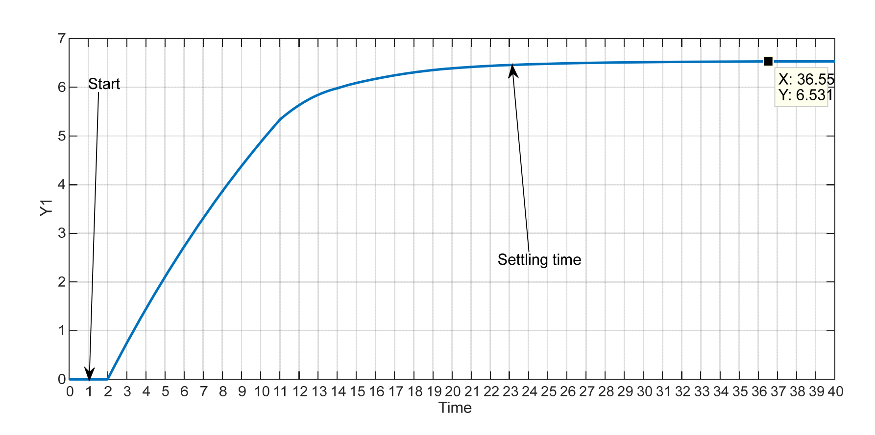
apply a 1-unit step change in $r1$ and plot $t$ against $y1$
from this step response, obtain the fopdt parameters (to be used in the next step)

Sequential loop closing example

from the step response of $y_1$ :
- delay: $\theta = 1$
- time constant: $\tau_p = \dfrac{23 - 2}{4} = 5.25$
- gain: $k_p = 6.53$

linearized model for loop 1:

$g'_{11} = \frac{6.53 \, e^{-s}}{5.25s + 1}$

Sequential loop closing example

design pid 1 using the linearized model $g'_{11}$

$g'_{11} = \frac{6.53 e^{-s}}{5.25s + 1}$

$g_{c1} = 0.4405 \left( 1 + \frac{1}{5.7s} + 0.456s \right)$

$gm = 9.92 \, db, \quad pm = 74.6^\circ$
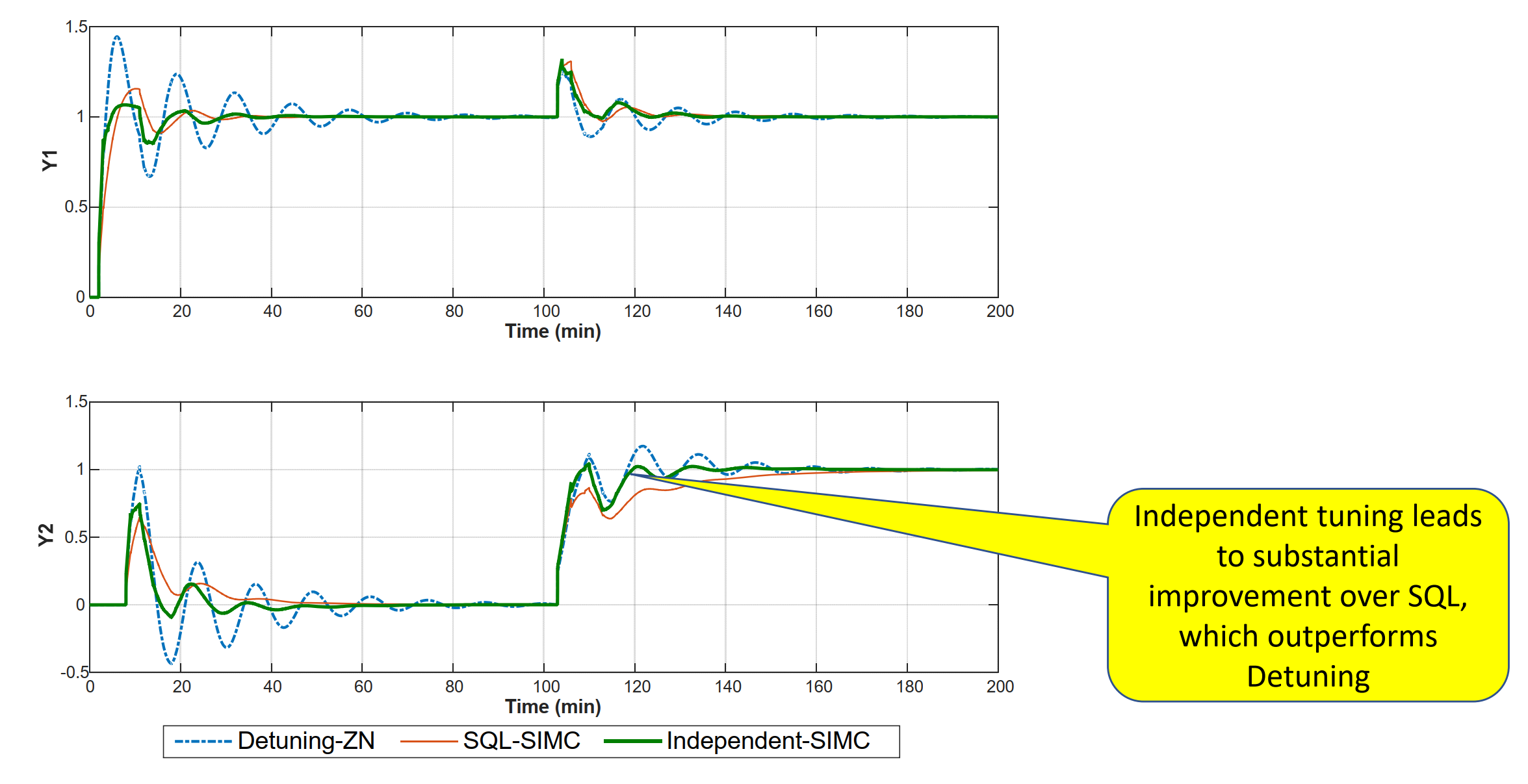
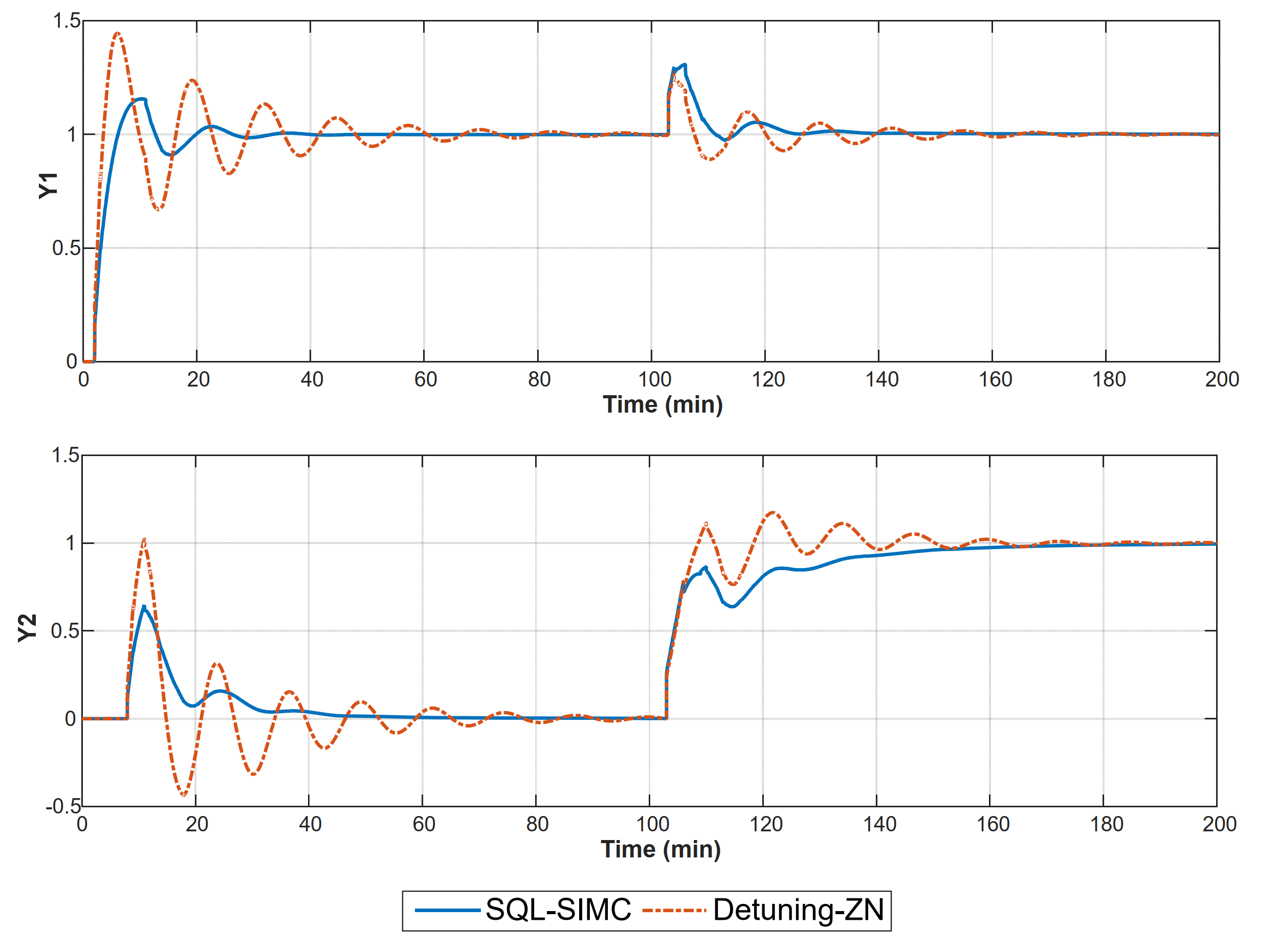
the plots show comparison between sql tuning and the previous detuning method
sql demonstrates substantial improvement in closed-loop performance compared to detuning

Independent tuning method

Independent tuning method relies on the Effective Open-Loop Transfer Function (EOTF)
For a 2×2 MIMO transfer function matrix:

$G = \begin{bmatrix} g_{11} & g_{12} \\ g_{21} & g_{22} \end{bmatrix}$
Reduce to decentralized form:

$G = \begin{bmatrix} g_{e11} & 0 \\ 0 & g_{e22} \end{bmatrix}$

EOTFs:

$g_{e11} = g_{11} - \frac{g_{12} g_{21}}{g_{22}}, \quad g_{e22} = g_{22} - \frac{g_{12} g_{21}}{g_{11}}$

Controllers $G_{c1}$ and $G_{c2}$ are designed independently based on $g_{e11}$ and $g_{e22}$
Existing SISO tuning formulas can be used
Next, we illustrate application of independent tuning for the Wood and Berry column example

Multi‐loop pid controllers for WB column – independent tuning method

Recall WB column transfer function:

$G = \begin{bmatrix} \dfrac{12.8 e^{-s}}{16.7s+1} & \dfrac{-18.9 e^{-3s}}{21s+1} \\ \dfrac{6.6 e^{-7s}}{10.9s+1} & \dfrac{-19.4 e^{-3s}}{14.4s+1} \end{bmatrix}$

Effective Open-Loop Transfer Functions (EOTFs):

$g_{e11} = \dfrac{12.8 e^{-s}}{16.7s+1} - \dfrac{\left( \dfrac{-18.9 e^{-3s}}{21s+1} \right) \left( \dfrac{6.6 e^{-7s}}{10.9s+1} \right)} {\dfrac{-19.4 e^{-3s}}{14.4s+1}}$

$g_{e11} = \dfrac{12.8 e^{-s}}{16.7s+1} - \dfrac{6.43 (14.4s+1) e^{-7s}}{(21s+1)(10.9s+1)}$

Multi‐loop pid controllers for WB column – independent tuning method

Approximation is required to simplify the EOTF
Equalize delays of main and coupling transfer functions
Assume general formula:

$g = \dfrac{k_p e^{-(\theta_1+\theta_2)s}}{(\tau_1 s+1)(\tau_2 s+1)} \;\; \approx \;\; \dfrac{k_p e^{-\theta_1 s}}{(\tau_1 s+1)(\tau_2 s+1)(\theta_2 s+1)}$
Applying to coupling transfer function:

$g_{e11} \approx \dfrac{6.43 (14.4s+1) e^{-s}}{(21s+1)(10.9s+1)(6s+1)}$
Overall EOTF for loop 1:

$g_{e11} = \left[ \dfrac{12.8}{16.7s+1} - \dfrac{6.43(14.4s+1)}{(21s+1)(10.9s+1)(6s+1)} \right] e^{-s}$
This simplified transfer functions can be used in Matlab Control System Designer since they contain only a single delay term

Multi‐loop pid controllers for WB column – independent tuning method

The second EOTF can be derived in the same manner

Overall EOTF for loop 2:

$g_{e22} = \left[ \dfrac{-19.4}{14.4s+1} + \dfrac{9.745(16.7s+1)}{(21s+1)(10.9s+1)(6s+1)} \right] e^{-3s}$
Controller Design using Skogestad IMC Tuning
- For $g_{e11}$ :
$G_{c1} = 0.775 \left( 1 + \dfrac{1}{8.5s} + 0.471s \right)$

$GM = 8.96 \, dB, \quad PM = 75.2^\circ$
- For $g_{e22}$ :
$G_{c2} = -0.16 \left( 1 + \dfrac{1}{9.3s} + 1.258s \right)$

$GM = 9.27 \, dB, \quad PM = 78.7^\circ$

Multi‐loop pid controllers for WB column – independent tuning method

Summary

Decentralized or multi-loop PID control is widely applied in process industries
Multi-loop control is often implemented at the regulatory layer, crucial for achieving stability
Proper controller pairing is essential in decentralized design to handle process interactions
Relative Gain Array (RGA) is used to address the configuration issue
Use steady-state RGA when transfer function dynamics are comparable
Use dynamic RGA when transfer function dynamics differ significantly

Correct pairing and RGA analysis are critical for robust and stable multi-loop control