Artificial Neural Networks

Advanced Modeling and Control

Introduction

• Artificial Intelligence (AI): systems capable of performing tasks that typically require human intelligence

  • Typical tasks: learning from experience, understanding natural language, recognizing patterns, solving problems, and making decisions

  • Encompasses techniques like machine learning, neural networks, natural language processing, and robotics

• Machine Learning (ML): A subset of artificial intelligence that involves training algorithms to make predictions or decisions based on data

  • Regression, Artificial Neural Networks (ANN), decision trees, and clustering

• Deep Learning (DL): A specialized subset of ML focused on neural networks with many layers (“deep”)

  • Excels at processing unstructured data like images, text, and audio

• Artificial Neural Networks (ANN): A specific model within ML, inspired by the human brain’s structure

  • Consists of layers of interconnected “neurons.”
  • Basic building block used in both traditional ML and deep learning

Introduction

• ANNs are a class of machine learning models inspired by the human brain’s structure and function. They consist of interconnected units called neurons, organized in layers

• Brains and computers operate fundamentally differently from each other

  • Brains: No CPU, lots of slightly smart memory cells
    • Recognizing faces, retrieving information based on partial descriptions, organizing information: The more info available, the better the brain operates
  • Computers: One very smart CPU, lots of extremely dumb memory cells
    • Arithmetic, deductive logic (e.g., \frac{p \rightarrow q, \; p}{\therefore q}), retrieving information based on arbitrary features

• The brain is composed of neurons

  • Neurons convey and transform information through electrical signals
  • Information in neurons is represented by “activation” (a scalar value)

• ANNs are constructed and implemented to model the human brain

Biological Neuron

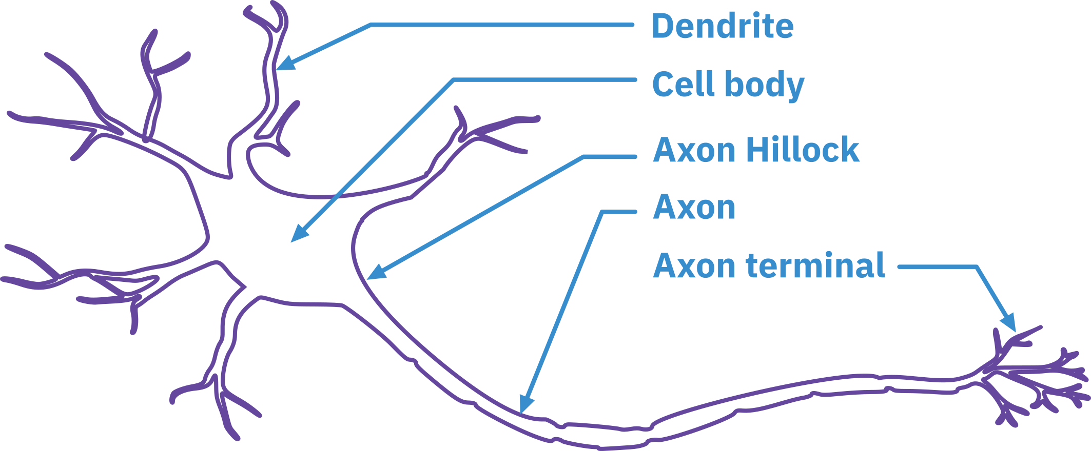
• Dendrite
  • Receives and integrates synaptic signals from other neurons
• Cell Body
  • Makes decisions based on integrated signals
• Axon
  • Passes signals to other neurons
  • Includes axon hillock (decision point) and axon collaterals (branches to nearby cells)

• Many neuron types exist.

• Interactions can be electrical or chemical.

• Different types of neuron connections (e.g., axodendritic, dendrodendritic).

• Key Characteristics of Neuronal Processing:

  • Slow signal propagation.
  • Large number of neurons (10^{10} – 10^{11}).
  • No central controller (CPU).
  • High connectivity (10^{4} connections per neuron).
  • Information conveyed by neuron firing rates (activation).

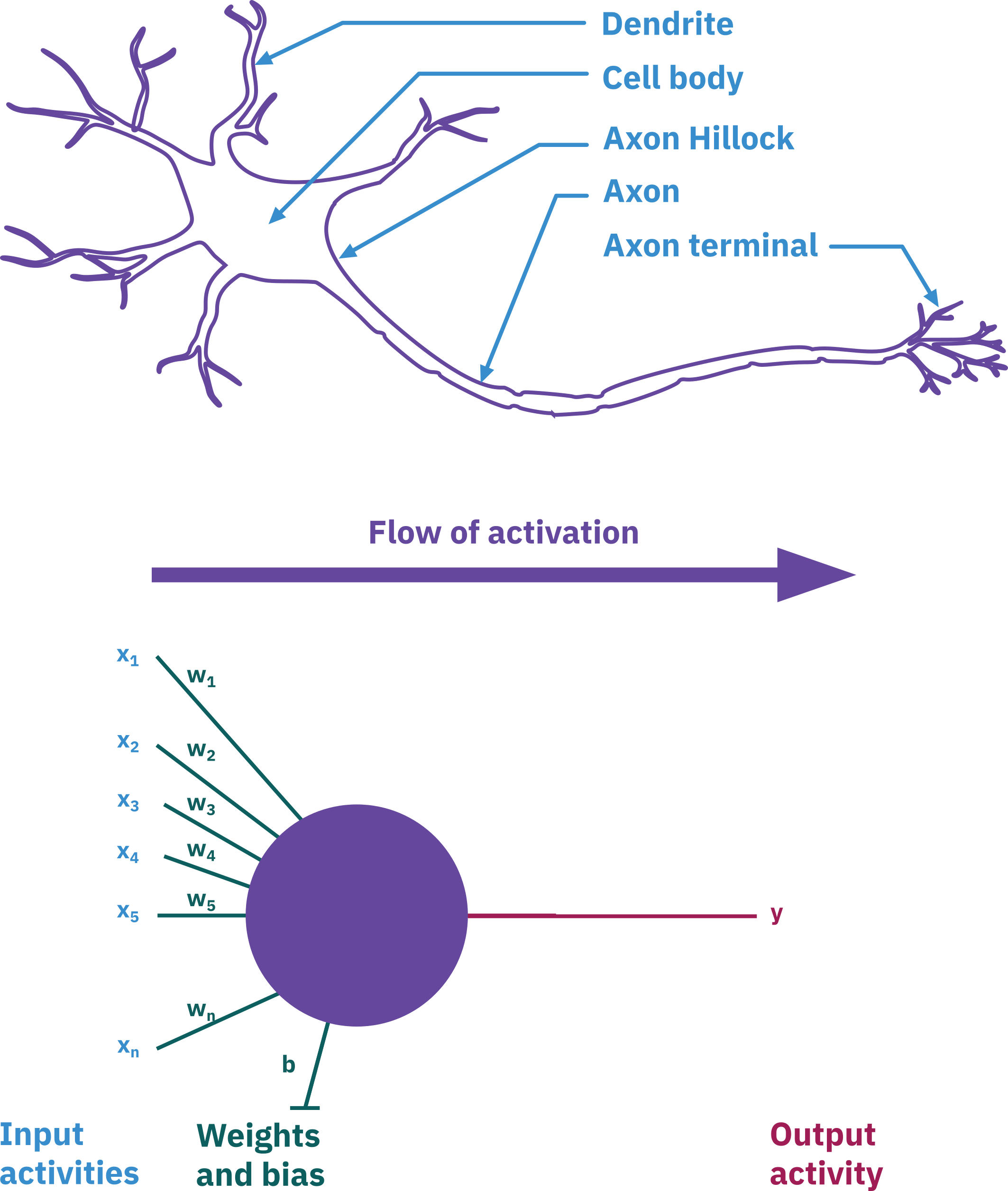
ANN basics: modeling single neuron

Universal Approximation Theorem

Any continuous function h(x) can be approximated by an ANN with one hidden layer, given appropriate non-linearity and sufficient neurons. Thus ANNs can model any complex, continuous function.

• Neurons receive multiple inputs.

• Inputs are modified by weights.

• Neurons sum weighted inputs.

• Neurons transmit output signals.

• Outputs connect to other neurons.

• Local Processing: Information is processed locally within the neuron.

• Distributed Memory: Short-term = signals; Long-term = weights.

• Learning: Weights adjust through experience.

• Flexibility: Neurons can generalize and are fault-tolerant.

Elements of neural networks

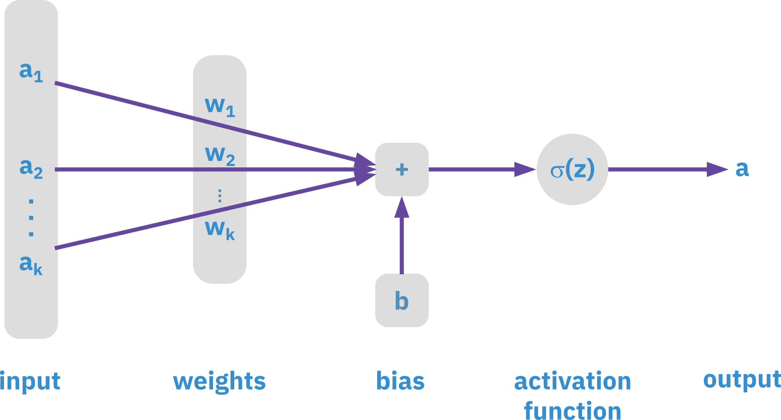
• ANNs consist of hidden layers with neurons (i.e., computational units)

• A single neuron maps a set of inputs into an output number, or f:R^K \rightarrow R

z = a_1 w_1 + a_2 w_2 + \ldots + a_k w_k + b; \qquad a = \sigma(z)

Elements of neural networks

ANN with one hidden layer and one output layer

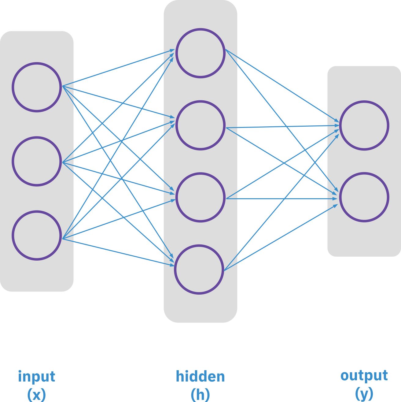
• Hidden layer

  h = \sigma (w_1 x + b_1)

• Output layer

  y = \sigma(w_2 h + b_2)

• Neurons: 6

  • Hidden layer: 4
  • output layer: 2

• Weights: 20

  • Hidden layer: 3 x 4
  • Output layer: 4 x 2

• Biases: 6

  • Hidden layer: 4
  • Output layer: 2

• Total 26 learning parameters

Activation function

• Mathematical function in neural networks determining the output of a neuron.

• Introduces non-linearity to model complex patterns.

• Without it, neural networks would only perform linear transformations.

• Common Activation Functions

  • Sigmoid: Outputs: 0 to 1, used in binary classification.

    \sigma(x) = \frac{1}{1 + e^{-x}}

  • ReLU (Rectified Linear Unit): Outputs: Input if positive; otherwise 0. Common in deep networks.

    f(x) = \text{max}(0, x)

  • Tanh (Hyperbolic Tangent): Outputs: -1 to 1, centers data around zero.

    \text{tanh}(x) = \frac{2}{1 + e^{-2x}} - 1

Important terminologies of ANNs

• Weights

  • Parameters that transform input data in the network; each connection has an associated weight.

  • Weights determine the influence of each input on the output; higher weights mean stronger influence.

• Bias

  • An additional parameter that shifts the activation function, helping the model fit the data better.

  • Similar to the y-intercept in a linear equation, it allows the function to adjust left or right.

• Threshold

  • The value at which a neuron’s activation function decides whether to fire (produce an output).

  • In binary threshold functions, if the weighted sum exceeds the threshold, the neuron activates (outputs 1); otherwise, it doesn’t (outputs 0).

Important terminologies of ANNs

• Learning Rate

  • Controls how much weights are adjusted in response to errors during training.
  • Determines step size in gradient descent; smaller values mean more precise adjustments but slower convergence.

• Momentum Factor

  • Added to the weight update formula to accelerate gradient descent and reduce oscillations.
  • Incorporates previous updates to smooth the optimization path, speeding up convergence and avoiding local minima.

• Loss function

  • Measures the difference between predictions and actual values.
  • Training aims to minimize this loss for better accuracy. Common types: Mean Squared Error (MSE) for regression, Cross-Entropy Loss for classification.

Training an ANN: Forward and Backpropagation

• Training

  • The model learns the relationship between input and output data (supervisory learning)
  • Weights and biases are fine-tuned during training. The goal is to minimize the error between predicted and actual outputs.

• Forward Propagation

  Passing input data through the network to produce an output, utilizing weights, biases, and activation functions.

• Backpropagation

  The process of refining the network by adjusting weights and biases based on the error, enabling the model to learn and improve over time (iterations).

• Adjusting weights and biases

  Move in the negative direction of the error (cost) function’s slope until a minimum error value is reached

  \Rightarrow Gradient descent

Gradient Descent

• Optimization algorithm used to minimize the cost function in machine learning

• Cost function (loss function or objective function)

  • Measures the difference between the predicted outputs and the actual target values.
  • Mean Squared Error (MSE): Common for regression tasks
  • Cross-Entropy Loss: Often used in classification tasks, it measures the difference between two probability distributions – the predicted probabilities and the actual labels

• Calculate the gradient (partial derivatives) of the cost function with respect to each parameter

• Adjust the parameters in the opposite direction of the gradient to decrease the cost function. Iterate until the cost function reaches a minimum

• Variants

  • Stochastic Gradient Descent (SGD): Uses a random subset of data per iteration to speed up computation.
  • Adaptive Gradient Descent: Adjusts step size for different data components (useful for text, image data).
  • Momentum Gradient Descent: Uses previous gradients to build momentum, accelerating convergence.

Overfitting

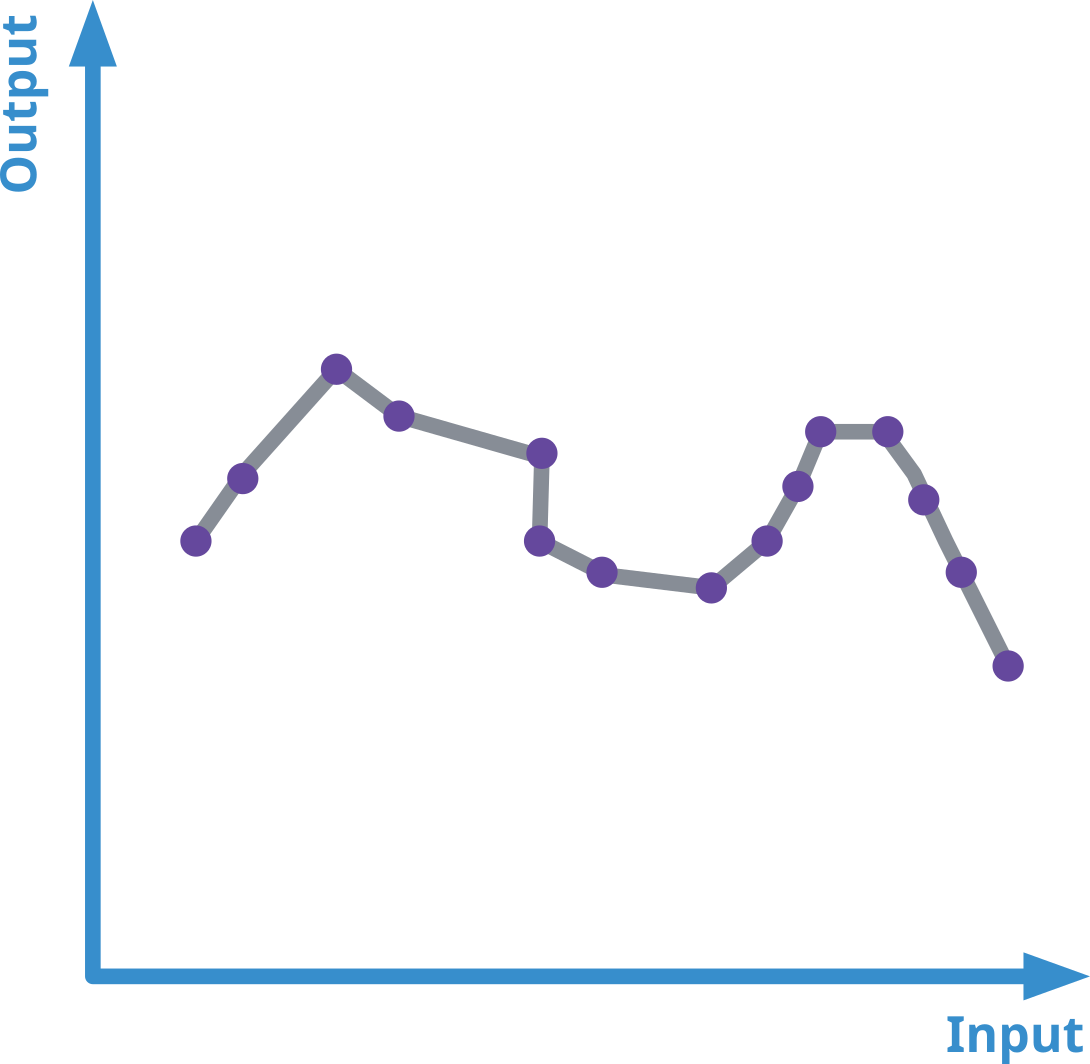
• Overfitting occurs when a machine learning model learns not only the underlying patterns in the training data but also the noise and random fluctuations.

• The model fits the training data too closely, capturing even the minor details and noise.

• The model performs very well on the training data but poorly on new, unseen data

• Causes

  • Too Complex Model: Using a model with too many parameters or features relative to the amount of training data.

  • Insufficient Training Data: When there isn’t enough data to represent the true underlying patterns, the model may learn noise as if it were a pattern.

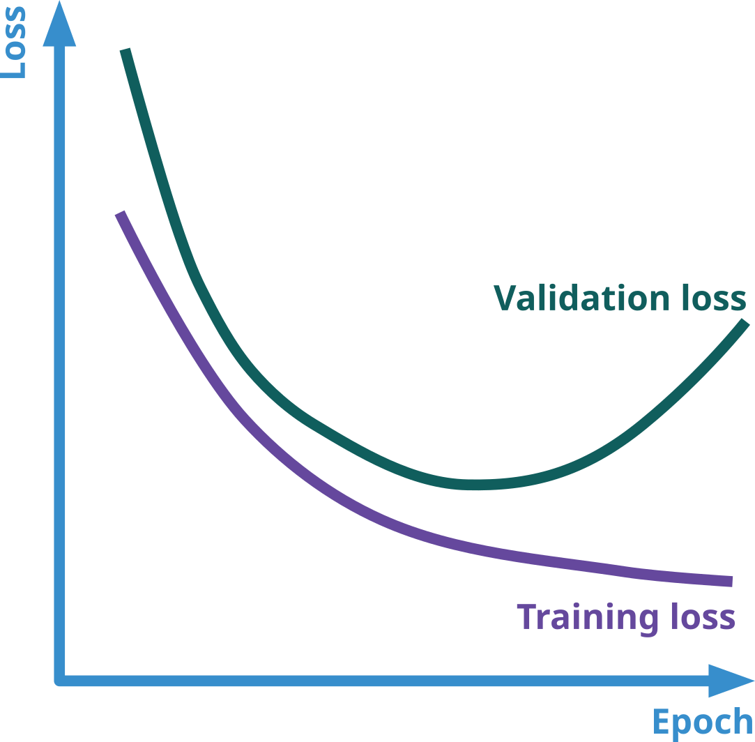
  • Too Long Training: Training the model for too many iterations, allowing it to adjust to even the smallest noise in the data.

Overfitting mitigation strategies

• Simplifying the Model: Reducing the number of features or parameters in the model.

• Cross-Validation: ensure the model generalizes well to unseen data.

  k-fold:

  • divide the data into k subset
  • Train the model k times. Each time one subset is used for validation and the rest are used for training
  • Average the results

• Regularization: Adding a penalty to the cost function for large coefficients

  • L1: Helps the model focus on the most important features by setting some weights to zero.
  • L2: Keeps all features but reduces the impact of any single feature by making all weights smaller.

• Early Stopping: Halting the training process when performance on a validation set starts to degrade, even if the training performance is still improving.

Network Architectures

• Perceptron & Feed-Forward Networks (FFN)

  Basic prediction tasks, such as property estimation, reaction rate predictions, and process optimization.

• Recurrent Neural Networks (RNN) & Long Short-Term Memory (LSTM)

  Modeling dynamic systems, time-series data, and sequential processes, such as reactor dynamics and control systems.

• Convolutional Neural Networks (CNN)

  Primarily in image analysis related to process monitoring (e.g., analyzing images from reactors, identifying patterns in images of materials).

• Autoencoders & Variational Autoencoders (VAE)

  Dimensionality reduction, feature extraction, fault detection, and process monitoring.

• Generative Adversarial Networks (GAN)

  Generating synthetic data for simulations, improving the robustness of models, and process optimization.

The neural network zoo

Summary

• ANNs are powerful tools for modeling complex, non-linear relationships in data.

• ANNs are applied to a wide range of chemical engineering problems, from static predictions to dynamic process control.

• Key Concepts:

  • Activation Functions: Introduce non-linearity to capture complex patterns (e.g., Sigmoid, ReLU, Tanh).
  • Training: Involves forward propagation (prediction) and backpropagation (learning from errors).
  • Optimization with Gradient Descent: Minimizes the error between predictions and actual values through iterative updates.

• Overfitting can be prevented by simplifying the model, using cross-validation, applying regularization, and early stopping to prevent overtraining

• Several network architectures exist

  \Rightarrow Successfully designing, training, and deploying ANNs often requires deep domain knowledge and experience in machine learning.