Principal Component Analysis
Advanced Modeling and Control
LDA Example
- Two-class dataset with overlapping Gaussian distributions.
- LDA finds a line (projection) that maximizes the separation.
- Classification is based on the projected values on w.
- Decision boundary is linear.


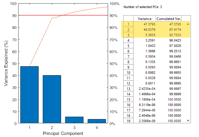
PCA analysis

Principal components show directions of the data that explain a maximal amount of variance
The larger the variance carried by a line, the larger the dispersion of the data points along it
Original data on the left with original coordinate x_1 and x_2
Variance of each variable graphically represented
Direction of the maximum variance i.e., principal component PC1 and PC2
Process modeling using PCA
Distillation column example
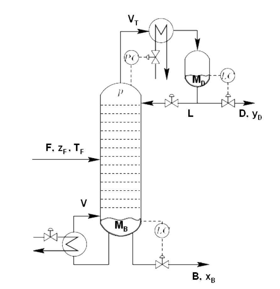
Separating a Methanol — Ethanol mixture
CVs: Y_D, X_B; MVs: D, B, L, V; DVs: F_T z
SISO control
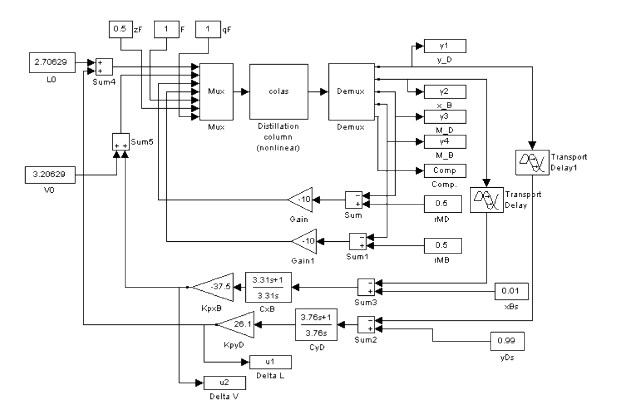
Model and data set incorporated in app
Workflow
- Phase I: Model steady state with PCA
- Phase II: Project new observations on model and detect deviation
Phase I: Model steady state with PCA
- Phase I: Model building to capture normal operating conditions
- No plant data \rightarrow use Simulink model to generate process data
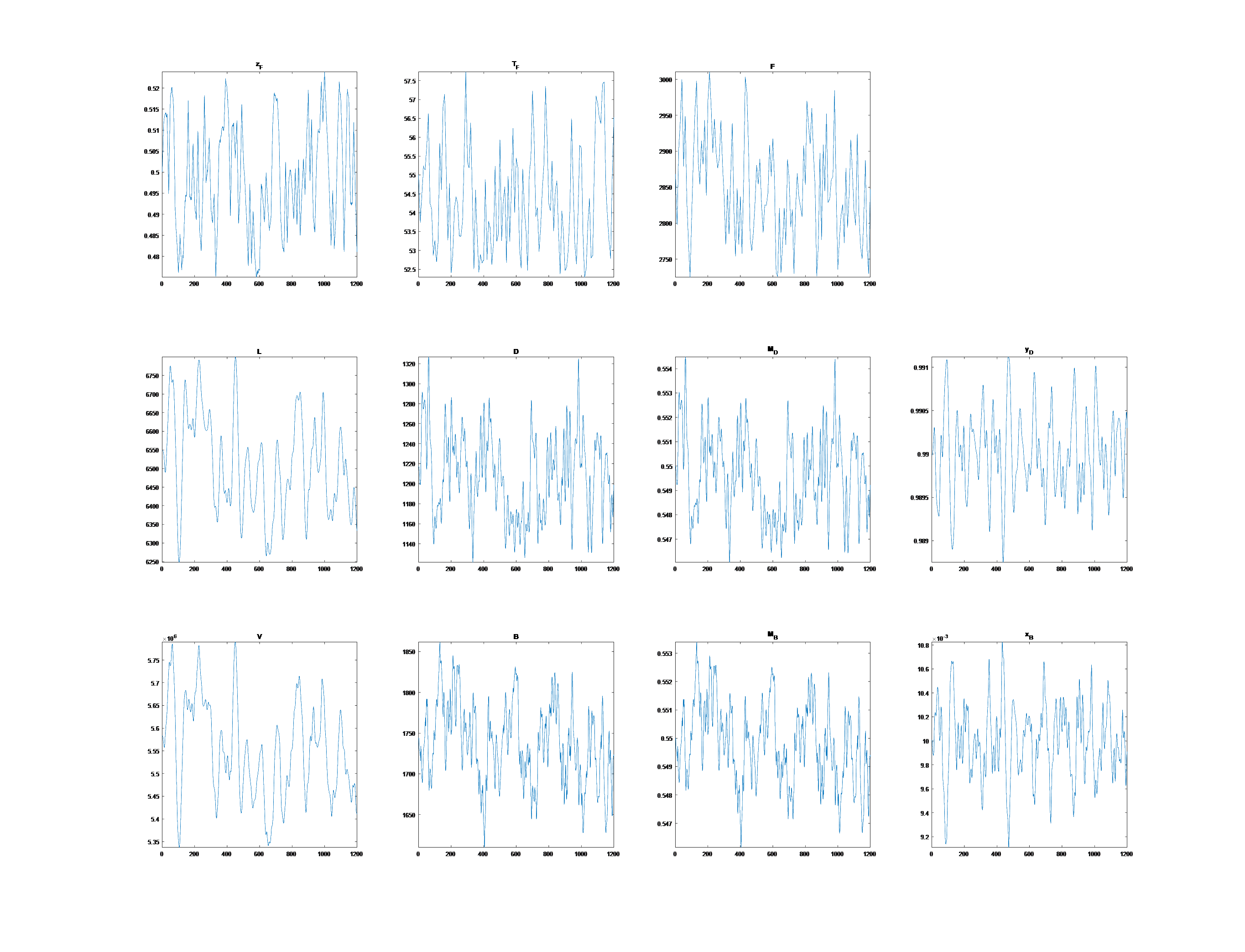
Phase I: Model steady state with PCA
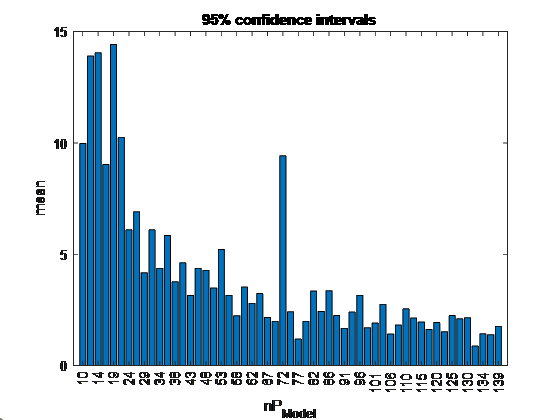
- Reduce size of data set
- Higher observations means better model but increases computing requirement
- Derive PCA model based on smallest data set that represents information in entire data set
- Select random subset
- Fit PCA model
- Compute percentage of out-of-control points
- If below threshold (5%), stop or else repeat above steps by increasing size of random subset

Phase I: Model steady state with PCA
Phase I: Model steady state with PCA
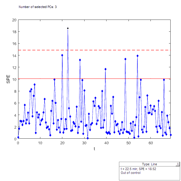
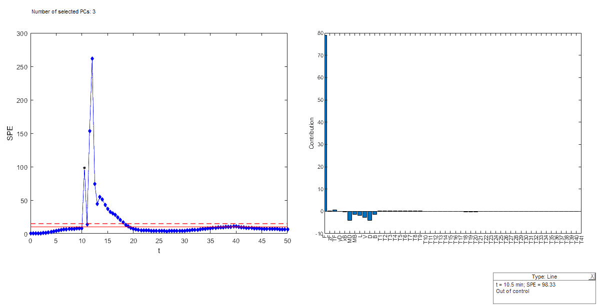
SPE control chart
- Measures the distance to the model
Hotelling’s T^2 control chart
- Measures if the projected observations are in NOC zone
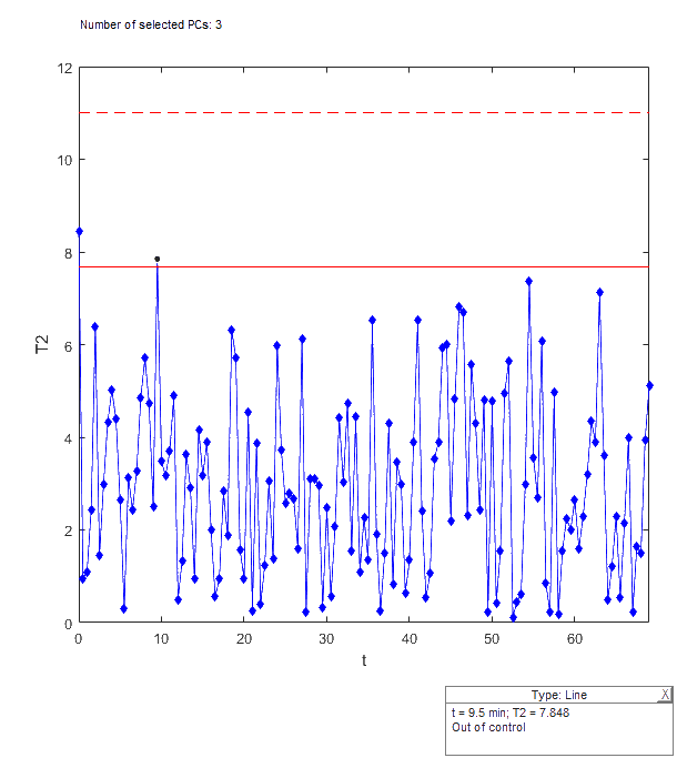
- Solid red line indicates 90% confidence interval; dashed red line indicates 95% confidence interval.
Phase II: Model exploitation
New ‘faulty’ data is pre-processed and projected onto the PCA model
If process is below control limits in both charts Process under control
If point is outside limits
- Check SPE chart and look at corresponding contribution plots
- Check T2 chart and look at corresponding contribution plots
Faults
Pl loop failure
Operating mode change
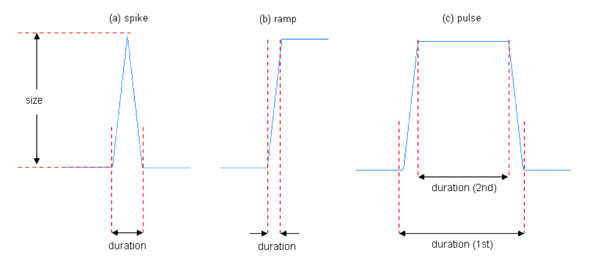
3 types of process disturbance: spike, ramp, pulse
![]()
Contribution chart
Shows how each original variable contributes to a particular principal component
Helps to identify which variables are most responsible for the patterns or outliers
Variables with higher contributions are those that have a stronger influence on the differentiation of the observations.
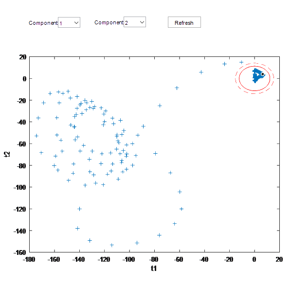
Scores
Score plot typically represents the data points projected onto the first two principal components.
Each point represents an observation (e.g., a sample or an experiment) in the reduced dimensionality space.
The score plot is used to identify patterns, groupings, or outliers in the data.
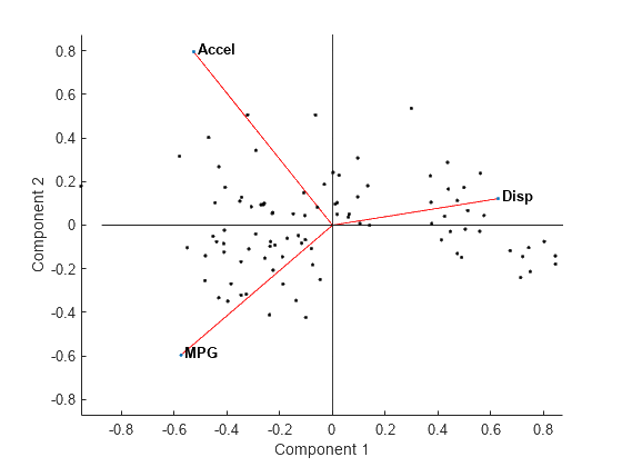
Biplot
The points in the biplot represent the samples projected onto the principal components (in PCA) or latent variables (in PLS).
The position of each point reflects how the sample is related to the components.
The vectors or arrows represent the original variables. The direction and length of each vector indicate the contribution of the variable to the components. Longer arrows suggest a stronger influence on the corresponding component. Variables that are closer to the origin have less influence on the components
Smaller angles between vectors suggest higher positive correlation, whereas angles close to 180° suggest a negative correlation.
Variable importance in projection (VIP) score
Identifying the most influential variables in the model
Shows the VIP scores, which are metrics that quantify the contribution of each variable to the model across all components
A common threshold is a VIP score of 1. Variables with VIP scores greater than 1 are generally considered significant contributors to the model, while those with scores below 1 may be considered less important.
Variables with high VIP scores are essential in explaining the variation in the dependent variable. They have a strong influence on the model’s predictions.
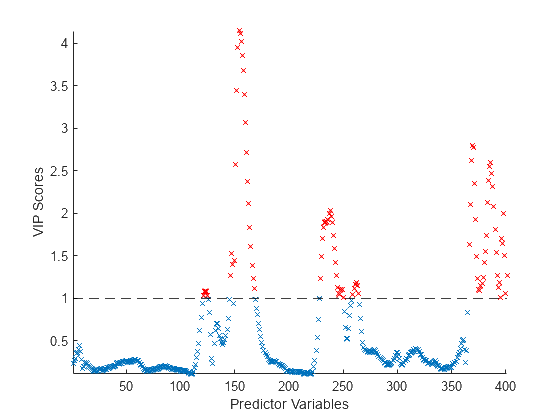
The VIP score plot can guide the selection of variables when refining a model, helping to focus on the most informative predictors.
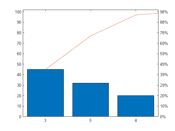
Pareto plot
Pareto principle (80/20 Rule): roughly 80% of the effects come from 20% of the causes.
The x-axis lists the different categories, arranged in descending order of their impact or frequency. Left y-axis shows the frequency, right y-axis shows the cumulative percentage.
Bars (Frequency/Impact): The bars represent the individual factors or categories.
- Ordered from the most significant (highest frequency or impact) to the least significant.
Cumulative Line: cumulative percentage of the total impact or frequency