Time series Modelling and analysis
Advanced Modeling and Control
What is Time Series?
- A time series is a sequence of observations recorded at successive points in time
- Each observation is ordered, meaning the position in time matters
- Data is often collected at regular intervals:
- Seconds, minutes, hours (process monitoring sensors)
- Days, months, years (economic, environmental, health data)
- Seconds, minutes, hours (process monitoring sensors)
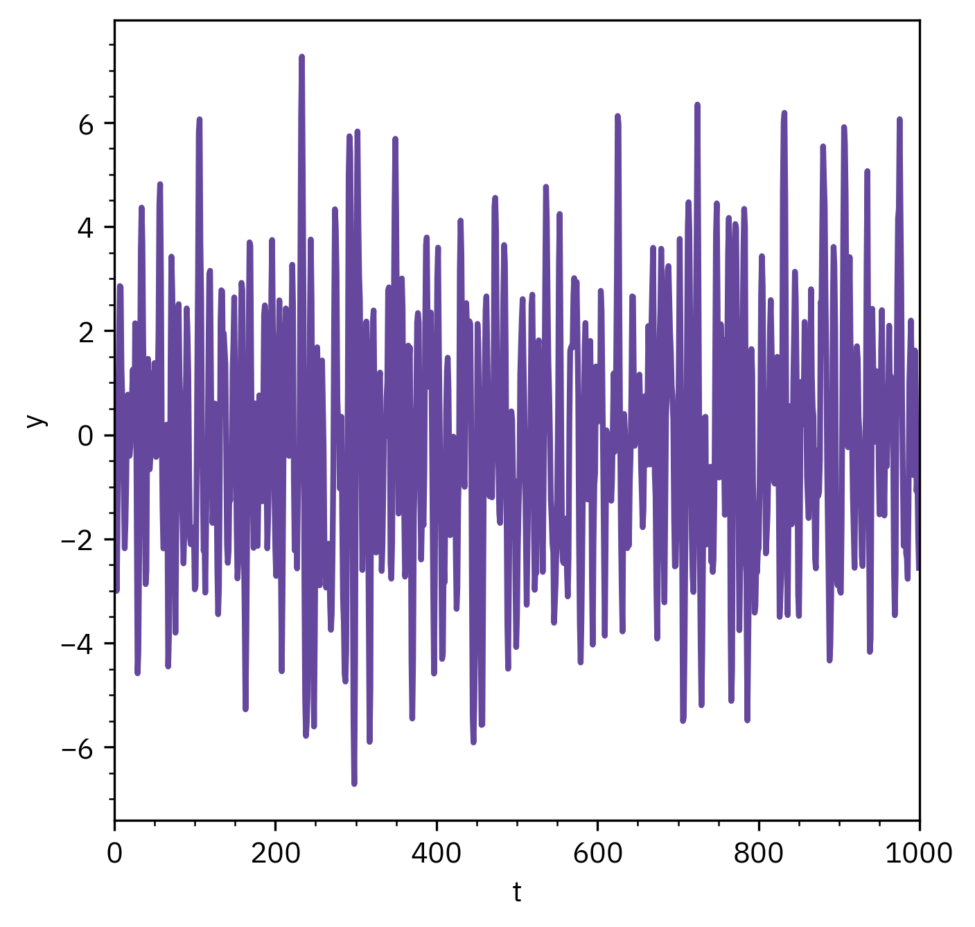
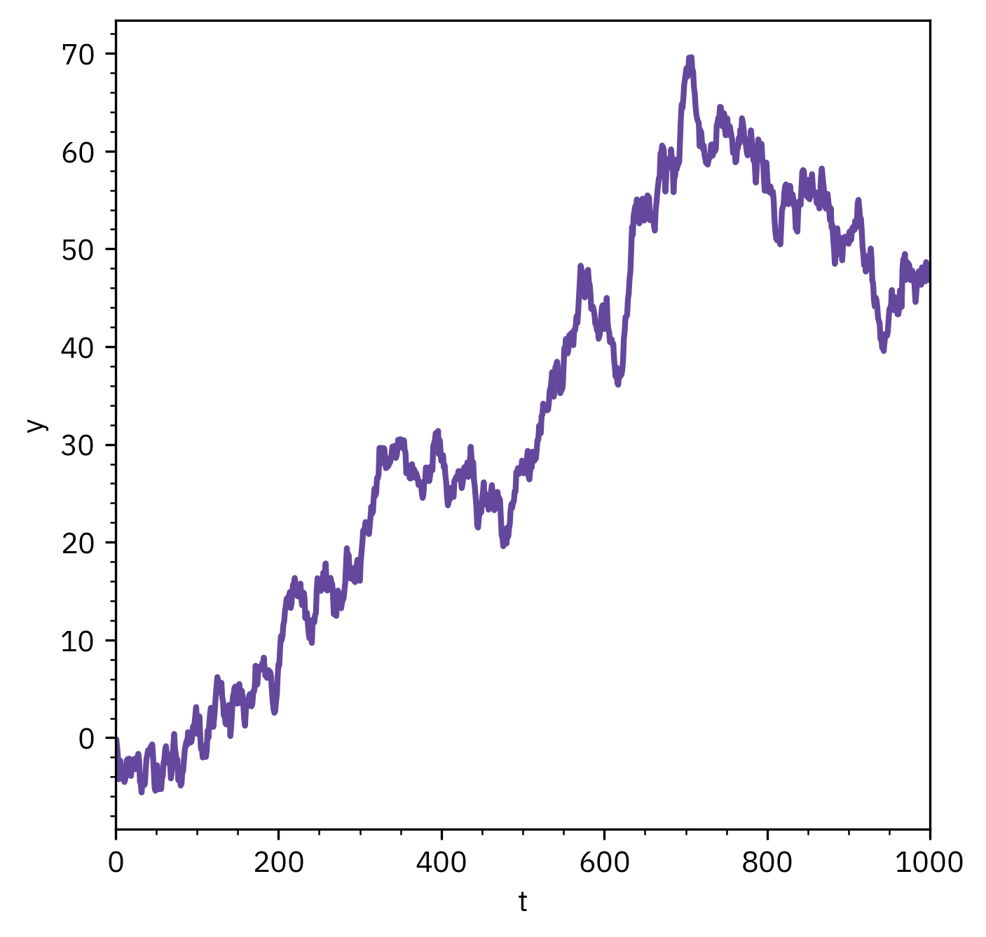
Stationary vs Non-stationary
Stationary series
- Mean and variance constant over time
- Fluctuates around a stable level
- Easier to model and forecast
Non-stationary series
- Mean or variance changes with time
- Shows trend, seasonality, or shifts
- Requires differencing or detrending
Time Series Representation
- Time series often large and high-dimensional
- Representation helps simplify analysis and comparison
- Common approaches:
- Raw series (original data)
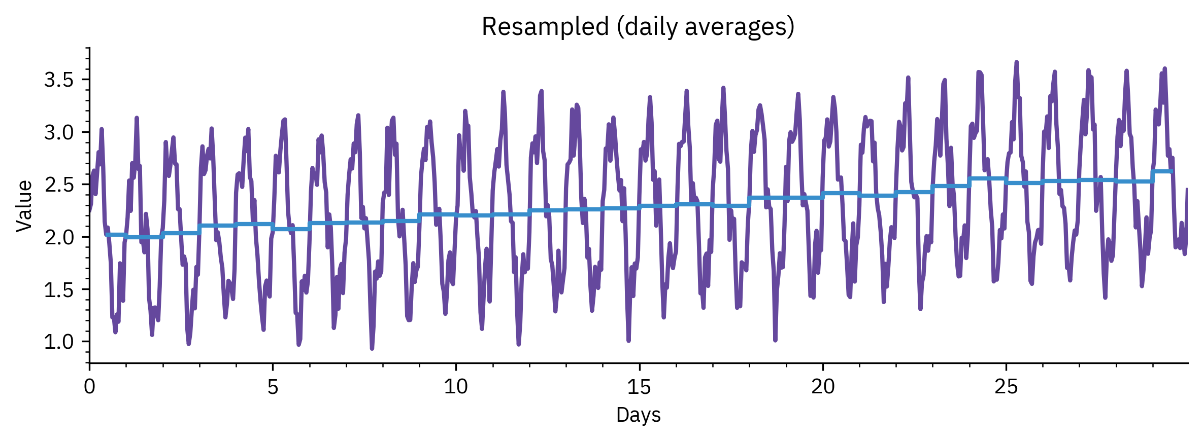
- Resampling (reducing data points, e.g., daily → monthly)
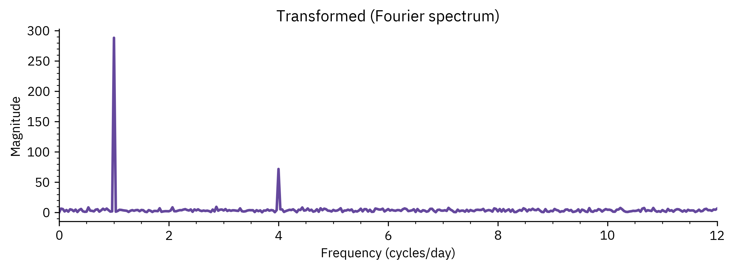
- Transformation (Fourier, wavelets, PCA)
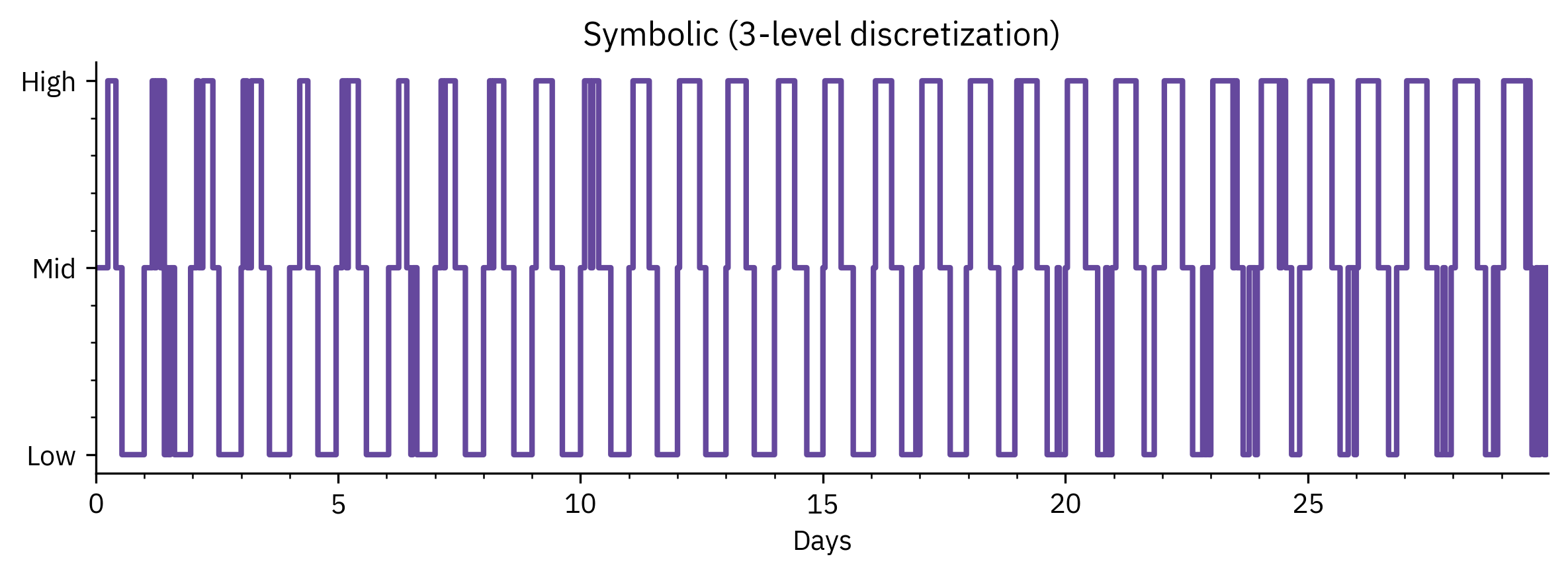
- Symbolic representation (grouping values into categories)
- Raw series (original data)
Benefits
- Reduces dimensionality while preserving essential patterns
- Enables efficient similarity search and clustering
- Provides basis for further tasks:
- Pattern discovery, Classification, Forecasting
Similarity Measures
- Used to compare two or more time series
- Important for:
- Clustering and classification
- Pattern discovery
- Anomaly detection
- Common measures:
- Euclidean distance
- Correlation-based distance
- Dynamic Time Warping (DTW) for misaligned series
- Euclidean distance
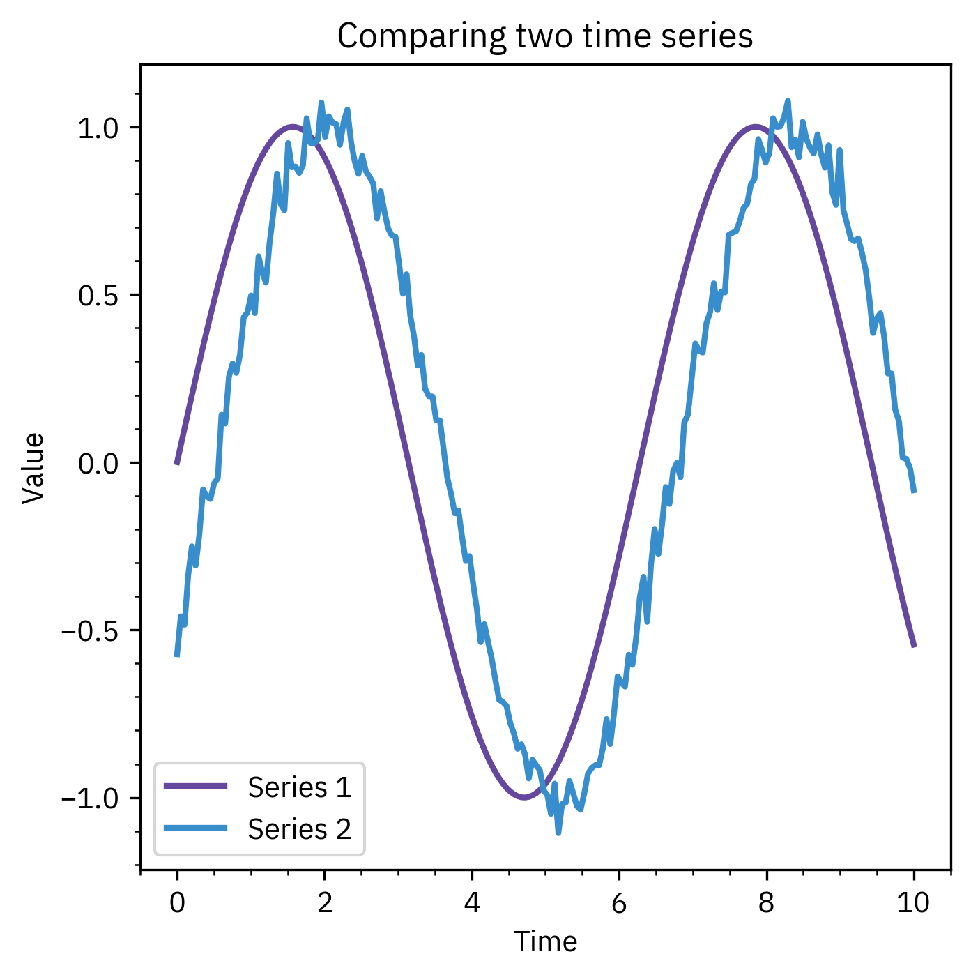
- Euclidean distance works if sequences are aligned
- DTW allows matching when sequences are stretched or shifted
- Correlation-based measures capture shape similarity
- Choice of similarity measure affects clustering, anomaly detection, and forecasting
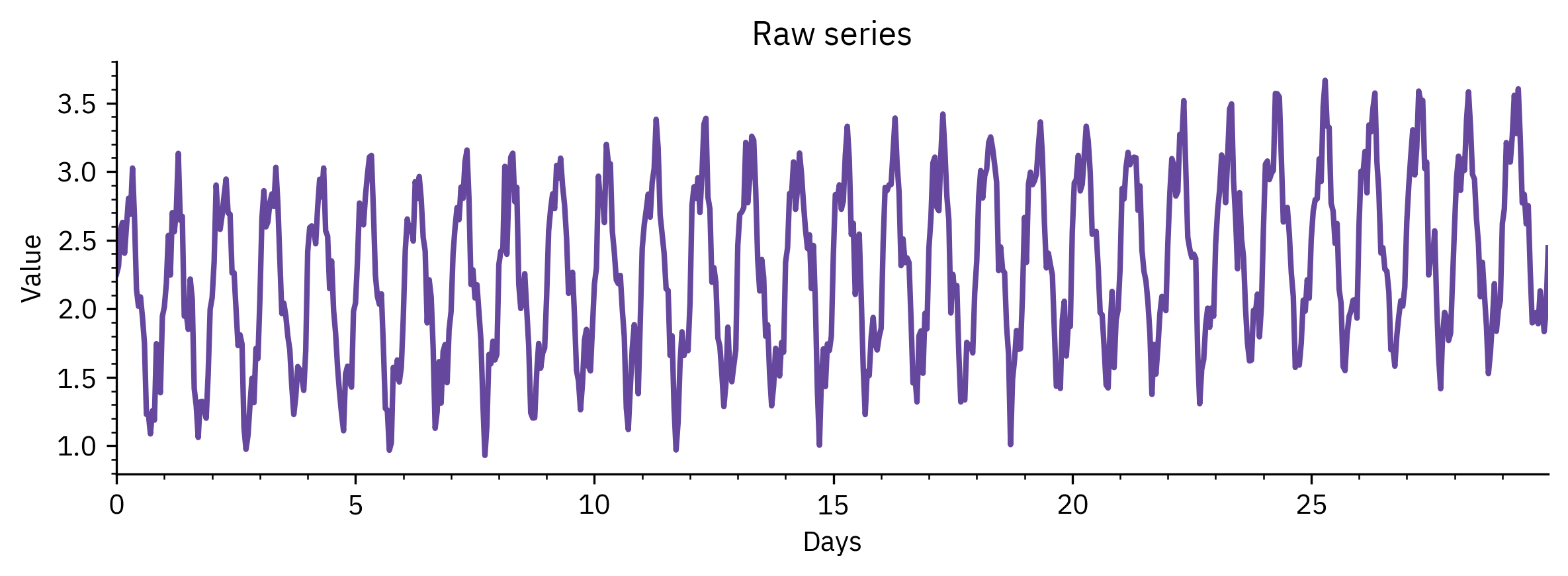
Characteristics of Time Series
- Temporal dependence: current values often depend on past values
- Directionality: useful for forecasting forward in time
- Patterns may include:
- Trend (long-term increase or decrease)
- Seasonality (repeated cycles, e.g., daily, monthly, yearly)
- Random fluctuations (noise)
- Trend (long-term increase or decrease)
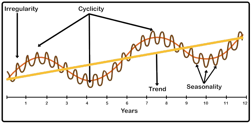
Time-Series Decomposition
- A time series can be expressed as the sum of underlying components
- Trend: long-term direction
- Seasonality: repeating cycles
- Cyclic variation: slower, irregular fluctuations
- Residual: noise or unexpected shocks
- Trend: long-term direction


Transfer Function Models
- Many physical processes can be represented by transfer functions in the Laplace domain
- Transfer function relates input → output dynamics
- Useful for:
- Capturing process gain, time constant, and delay
- Providing a baseline for time-series model comparison
- Often estimated from input–output data (system identification)
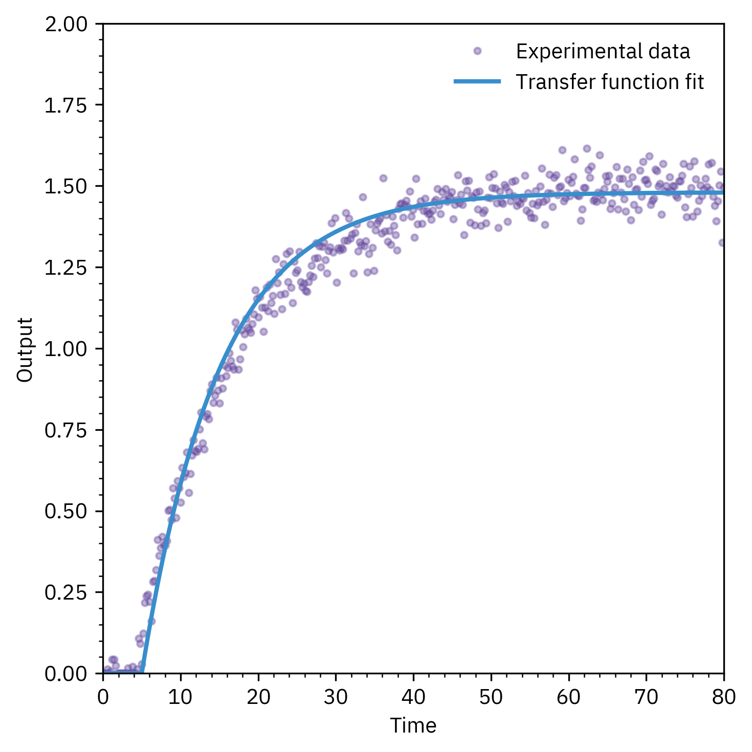
Transfer Functions as a Starting Point
- Physics-based intuition: order, delay, stability
- Provides initial guess for data-driven models (ARX, ARMAX)
- Bridges between first-principles modeling and time-series modeling
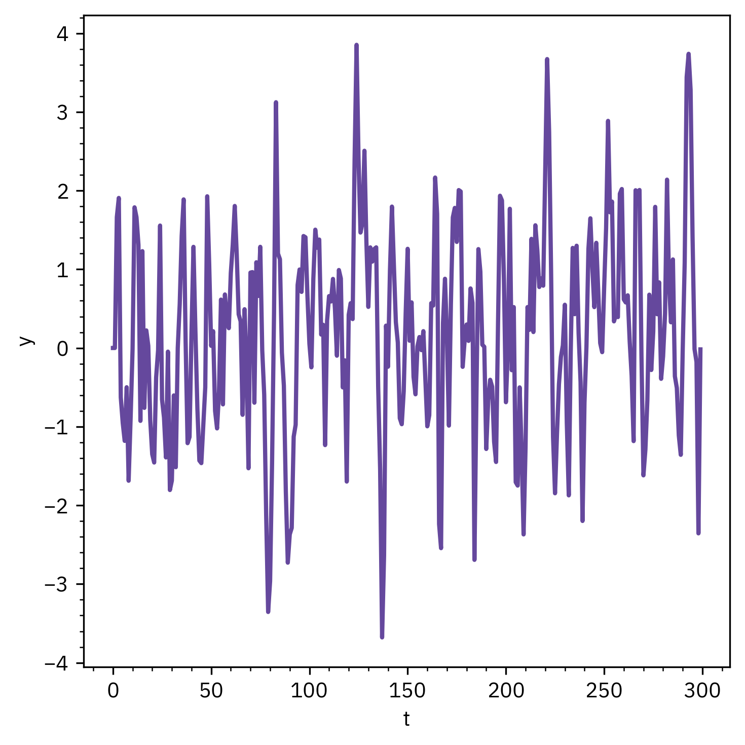
Autoregressive (AR) Models
- Concept
- Current value depends on a linear combination of past values
- AR(p):
y_t = \phi_1 y_{t-1} + \phi_2 y_{t-2} + \dots + \phi_p y_{t-p} + e_t - Captures short-term correlations in stationary data
- Current value depends on a linear combination of past values
- MATLAB
ar(data, order)estimates AR model
- Order selection via AIC / FPE
- Applications
- Forecasting short horizon
- Identifying dominant lags
- Noise modeling in ARMAX
- Forecasting short horizon
ARIMA Models
- ARIMA = Autoregressive Integrated Moving Average
- Extends ARMA for non-stationary series
Integration differencing step
\nabla y(t) = y(t) - y(t-1)
Makes the series stationary before ARMA modeling
- Interpretation
- AR: memory of past values
- I: removes trends and seasonality
- MA: corrects random shocks
- AR: memory of past values
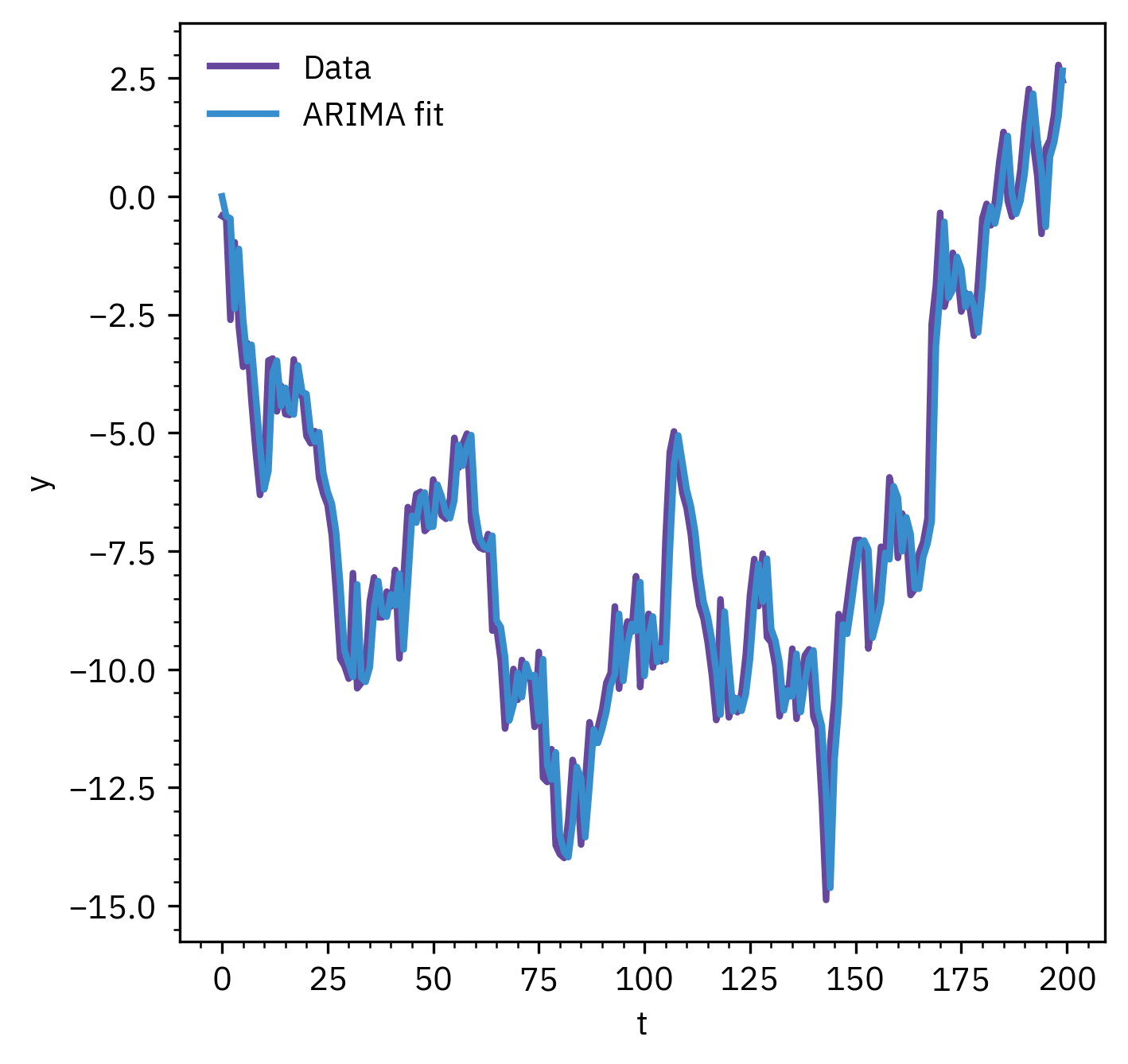
MATLAB
m = arima(p,d,q)
p = AR order; d = number of differences (integration order); q = order of MA part