AMC | Advanced Modeling and Control – Time series Modelling and analysis

Outline

Introduction & Motivation
Basics of Time Series
Transfer Function Models
Autoregressive (AR) Models
- ARX Models
- ARMAX Models
- ARMA/ARIMA Models
Model Evaluation & Selection
Summary & Reflection

What is Time Series?

A time series is a sequence of observations recorded at successive points in time
Each observation is ordered, meaning the position in time matters
Data is often collected at regular intervals:
- Seconds, minutes, hours (process monitoring sensors)
- Days, months, years (economic, environmental, health data)

Importance

Provides patterns and forecasts to support decisions
Anticipates specification violations in process industries
Typical applications:
- Process control
- Energy demand forecasting
- Equipment health monitoring
- Economic and financial trends
- Climate and agriculture planning
- Public health surveillance

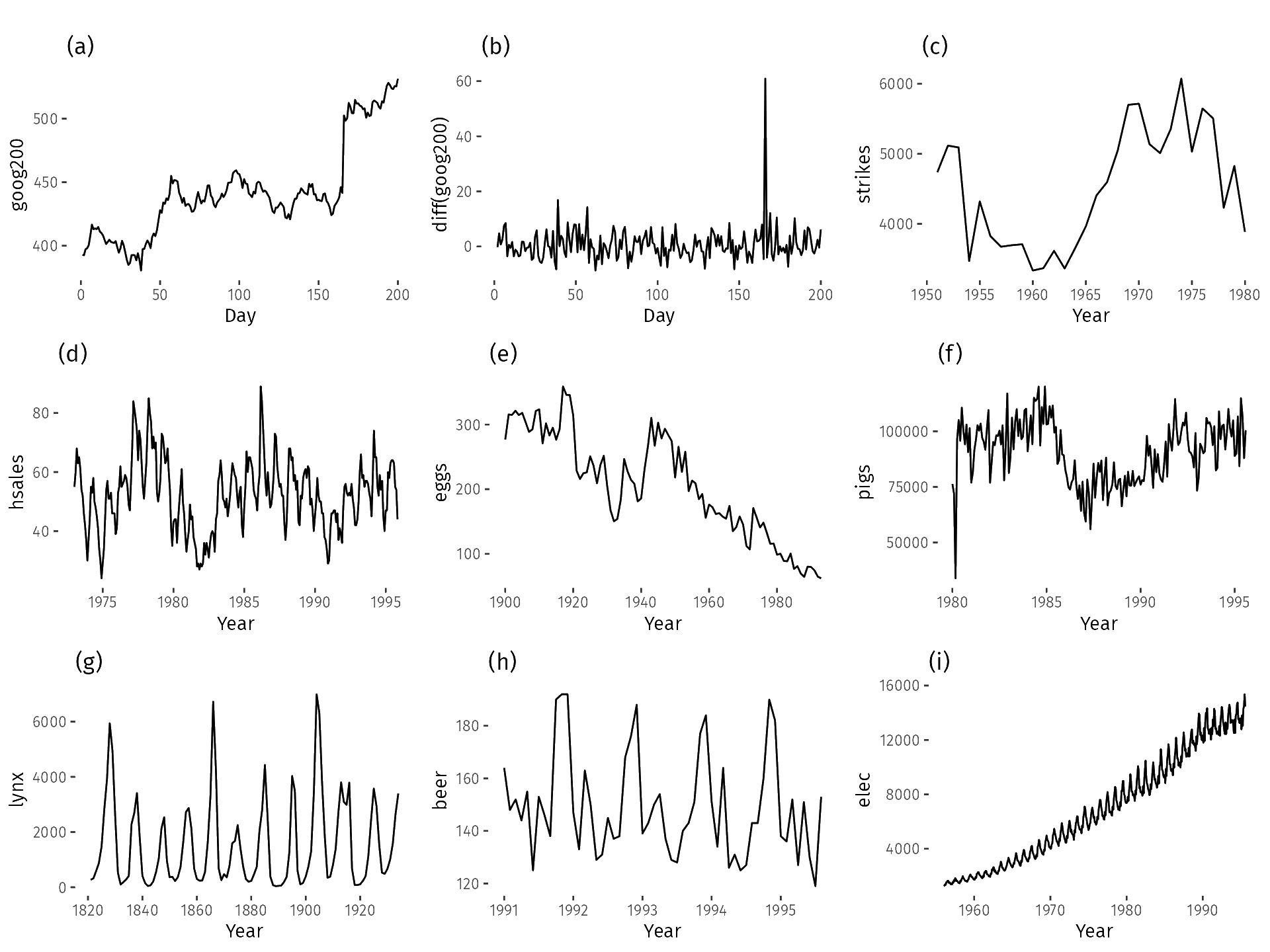
Stationary vs Non-stationary

Stationary series

Mean and variance constant over time
Fluctuates around a stable level
Easier to model and forecast

Non-stationary series

Mean or variance changes with time
Shows trend, seasonality, or shifts
Requires differencing or detrending

Time Series Representation

Time series often large and high-dimensional
Representation helps simplify analysis and comparison
Common approaches:
- Raw series (original data)
- Resampling (reducing data points, e.g., daily → monthly)
- Transformation (Fourier, wavelets, PCA)
- Symbolic representation (grouping values into categories)

Benefits

Reduces dimensionality while preserving essential patterns
Enables efficient similarity search and clustering
Provides basis for further tasks:
- Pattern discovery, Classification, Forecasting

Similarity Measures

Used to compare two or more time series
Important for:
- Clustering and classification
- Pattern discovery
- Anomaly detection
Common measures:
- Euclidean distance
- Correlation-based distance
- Dynamic Time Warping (DTW) for misaligned series

Euclidean distance works if sequences are aligned
DTW allows matching when sequences are stretched or shifted
Correlation-based measures capture shape similarity
Choice of similarity measure affects clustering, anomaly detection, and forecasting

Characteristics of Time Series

Temporal dependence: current values often depend on past values
Directionality: useful for forecasting forward in time
Patterns may include:
- Trend (long-term increase or decrease)
- Seasonality (repeated cycles, e.g., daily, monthly, yearly)
- Random fluctuations (noise)

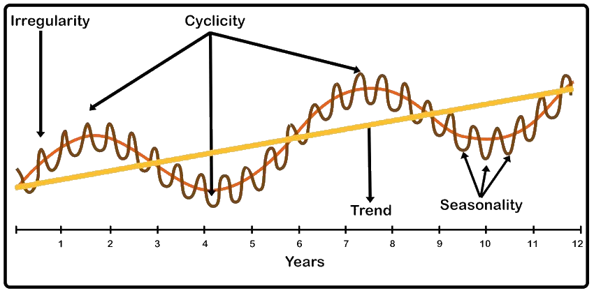
Time-Series Decomposition

A time series can be expressed as the sum of underlying components
- Trend: long-term direction
- Seasonality: repeating cycles
- Cyclic variation: slower, irregular fluctuations
- Residual: noise or unexpected shocks

Mining in Time Series

Goal: discover hidden information or patterns
Common tasks:
- Pattern discovery and clustering
- Classification (e.g., healthy vs faulty sensor data)
- Rule discovery (if X happens, Y follows)
- Summarization and anomaly detection

These tasks often rely on similarity measures, representation, and decomposition.

What Do We Mean by Modelling?

A model is a simplified description used to explain and predict data
Two perspectives:
- Structural: parameters have physical meaning (equation / transfer function)
- Data-driven: parameters capture patterns (e.g., neural network)
What models enable: simulation, forecasting, pattern recognition

Structural vs Data-Driven Models

Structural models

Based on physical laws and first principles
Parameters have physical interpretation
Examples:
- Transfer functions
- Differential equations

Pros: interpretability, extrapolation
Cons: need detailed knowledge

Data-driven models

Based on observed data patterns
Parameters capture correlations, not physics
Examples:
- AR, ARX, ARMAX
- Neural networks

Pros: flexible, captures complex patterns
Cons: less interpretable, may overfit

Transfer Function Models

Many physical processes can be represented by transfer functions in the Laplace domain
Transfer function relates input → output dynamics
Useful for:
- Capturing process gain, time constant, and delay
- Providing a baseline for time-series model comparison
Often estimated from input–output data (system identification)

Transfer Functions as a Starting Point

Physics-based intuition: order, delay, stability
Provides initial guess for data-driven models (ARX, ARMAX)
Bridges between first-principles modeling and time-series modeling

Activity 1: Estimating Transfer Function Models for a Heat Exchanger.

Autoregressive (AR) Models

Concept
- Current value depends on a linear combination of past values
- AR(p):
  $y_t = \phi_1 y_{t-1} + \phi_2 y_{t-2} + \dots + \phi_p y_{t-p} + e_t$
- Captures short-term correlations in stationary data
MATLAB
- ar(data, order) estimates AR model
- Order selection via AIC / FPE
Applications
- Forecasting short horizon
- Identifying dominant lags
- Noise modeling in ARMAX

Autoregressive (AR) Models

Present value depends on past values in discrete time
General AR(n):

$y_t = c + \sum_{i=1}^n \alpha_i y_{t-i} + \varepsilon_t$
- Where: $c$ : constant; $\alpha_i$ : AR coefficients; $n$ : model order; $\varepsilon_t$ : white noise
Example for AR(2):

$y_t = c + \alpha_1 y_{t-1} + \alpha_2 y_{t-2} + \varepsilon_t$
Properties of AR models
- Short-term memory, good for capturing autocorrelation
- Flexible building block for ARX, ARMAX, ARIMA

AR model with backshift operator $z^{-k}$

AR(2) in operator notation:

$y_t = c + \alpha_1 y_{t-1} + \alpha_2 y_{t-2} + \varepsilon_t$

can be written as

$(1 + \alpha_1 z^{-1} + \alpha_2 z^{-2}) y_t = c + \varepsilon_t$

$y_t = \frac{c + \varepsilon_t}{1 + \alpha_1 z^{-1} + \alpha_2 z^{-2}} \,=\, \frac{c + \varepsilon_t}{A(z)}$
Interpretation
- The AR model acts like a filter that takes in random noise and produces the series.
- The filter has only poles (all-pole system), so the effect of a shock gradually fades but never ends completely (infinite impulse response, IIR).
- In contrast, some models have responses that die out completely after a fixed time (finite impulse response, FIR).

In-class Activity 2

Fit an AR model to Australia COVID-19 infection data (Australia_covid_cases.xlsx) and evaluate order selection.

ARX Models

ARX: Autoregressive with Exogenous Input
Exogenous Input
- Many processes are driven by outside factors (inputs, e.g. manipulated variables, disturbances)
- In a distillation column, the feed composition or coolant flow are exogenous inputs that affect the impurity (output).
- In finance, the interest rate might be an exogenous input affecting stock prices.
👉 Exogenous input = something external you can measure and that drives the system.
Why ARX?
- AR models only use past outputs → good for forecasting trends
- ARX extends AR by including the exogenous inputs explicitly

ARX Model

Structure

$A(q^{-1}) y(t) = B(q^{-1}) u(t-n_k) + e(t)$ - $A(q^{-1})$ : polynomial in past outputs
- $B(q^{-1})$ : polynomial in past inputs
- $n_k$ : input delay
- $e(t)$ : noise

Interpretation
- Captures cause–effect between input and output
- Useful for system identification with I/O data

MATLAB

m = arx(data, [na nb nk])
where na = AR order, nb = input order, nk = input delay.

Activity 3: Develop an ARX Model for a Given Transfer Function

ARMA Models

ARMA: Autoregressive Moving Average
- AR models capture dependence on past outputs
- But sometimes random shocks persist for several steps (noise is not white)
- ARMA = AR + MA, adds a moving average (MA) term for noise

Structure

$A(q^{-1}) y(t) = C(q^{-1}) e(t)$ - $A(q^{-1})$ : polynomial in past outputs
- $C(q^{-1})$ : polynomial in past noise (MA part); $e(t)$ : white noise

Interpretation
- Models a stationary time series without external input
- Captures both memory in outputs and persistence in shocks
- Building block for ARIMA models (to handle non-stationarity)

MATLAB

m = arima(p,0,q)
where p = AR order, q = MA order.
Use estimate(m, data) to fit.

ARMAX Models

ARMAX: Autoregressive Moving Average with Exogenous Input
- ARX models assume the disturbance is white noise
- In practice, noise often has its own dynamics (colored noise)
- ARMAX extends ARX by adding a moving average (MA) term for noise

Structure

$A(q^{-1}) y(t) = B(q^{-1}) u(t-n_k) + C(q^{-1}) e(t)$ - $A(q^{-1})$ : past outputs; $B(q^{-1})$ : past inputs (exogenous input)
- $C(q^{-1})$ : noise dynamics (MA part); $n_k$ : input delay

Interpretation
- Captures both input–output dynamics and structured noise
- More flexible and realistic than ARX
- Often needed when residuals of ARX show correlation

ARIMA Models

ARIMA = Autoregressive Integrated Moving Average
Extends ARMA for non-stationary series
- Integration differencing step
  
  $\nabla y(t) = y(t) - y(t-1)$
- Makes the series stationary before ARMA modeling
Interpretation
- AR: memory of past values
- I: removes trends and seasonality
- MA: corrects random shocks

MATLAB

m = arima(p,d,q)
p = AR order; d = number of differences (integration order); q = order of MA part

Activity 4: Iron Ore Prices – ARIMA Modeling

Model Evaluation and Selection

Many possible models → need criteria to choose the best one
Avoid overfitting (too complex) and underfitting (too simple)
Common criteria
- Residual analysis (should look like white noise)
- Goodness of fit (%) to validation data
- Information criteria (Akaike information criteria (AIC), Final prediction error (FPE))
- Prediction accuracy (on test data)
Best practice
- Compare several models with different orders
- Choose the simplest model that explains the data well
- Validate with unseen (test) data if available

In MATLAB

goodnessOfFit
compare(data, model1, model2, ...) → compare fit visually
aic, fpe → return information criteria
resid(data, model) → check residuals

Summary

Time-series data can be broken into components: trend, seasonality, cyclic variation, and residuals
Models help us explain and predict time-series behavior
- AR models: depend on past outputs
- ARX models: extend AR by including exogenous inputs
- ARMA/ARMAX: combine autoregression with moving average, noise modeling
- ARIMA: adds differencing for non-stationary data
Model evaluation and selection
- Check residuals (should look like white noise)
- Use metrics like AIC, FPE, fit percentage
- Validate using unseen data

📌 Different models suit different needs — forecasting, simulation, or understanding system dynamics.