Recap: Basics of Process Control and Modelling

Advanced Modeling and Control

Table of contents

• Why process control
• Fundamentals of process modeling
• Dynamic Behavior of Processes
• Feedback Control Systems

Why process control

• Importance of process analysis and control
• Process control objectives
• Hirarchy of process control activities
• Overview of control system design

Importance of process analysis and control

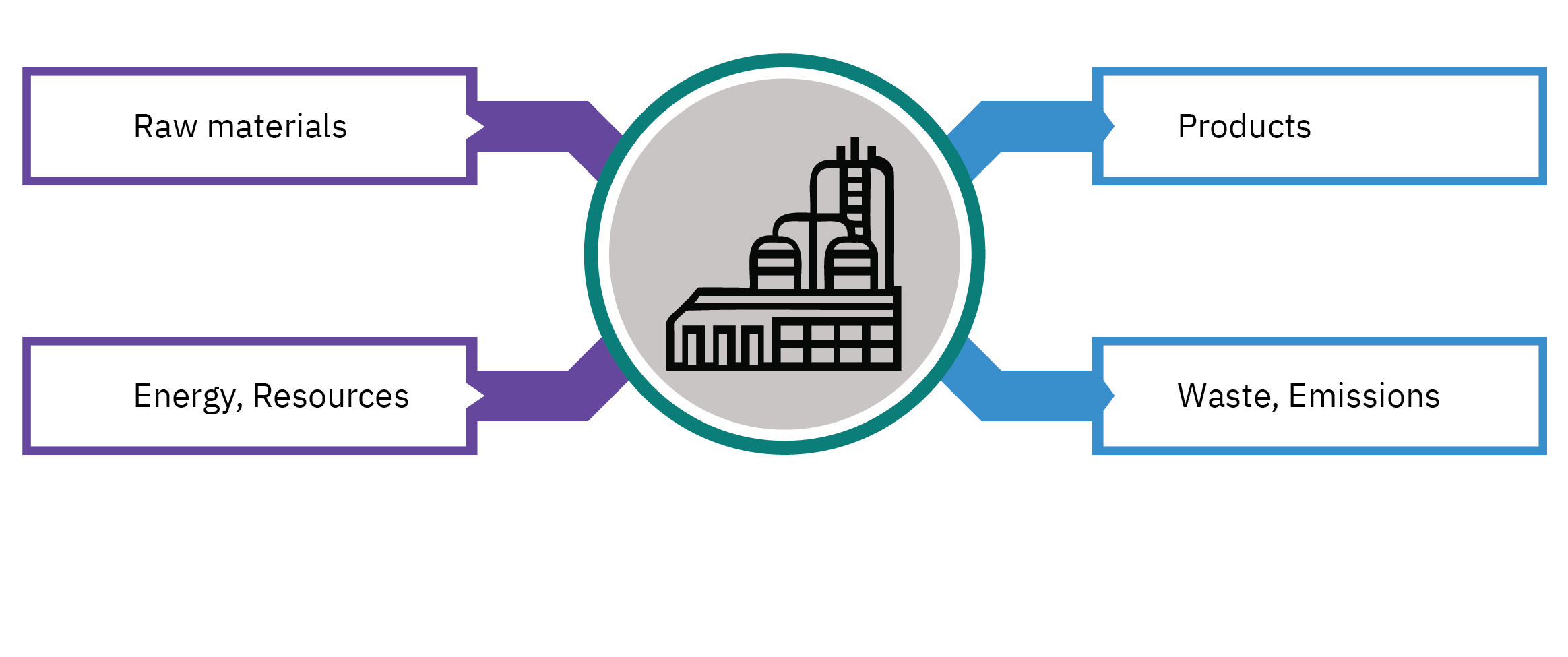
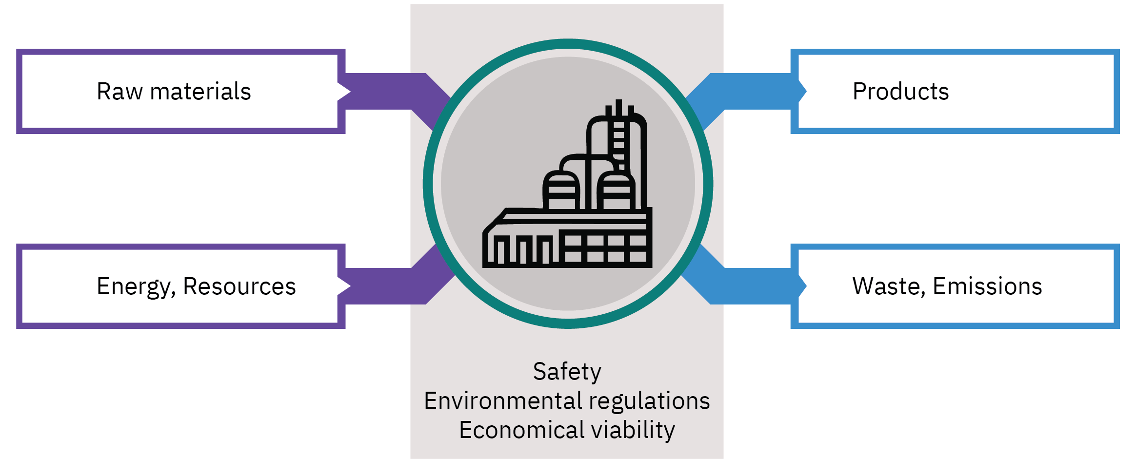
• Optimal process operations require efficient and effective control
• Control systems and advanced algorithms are deployed to monitor, regulate, and optimize the process variables.

Process System, Input and Output

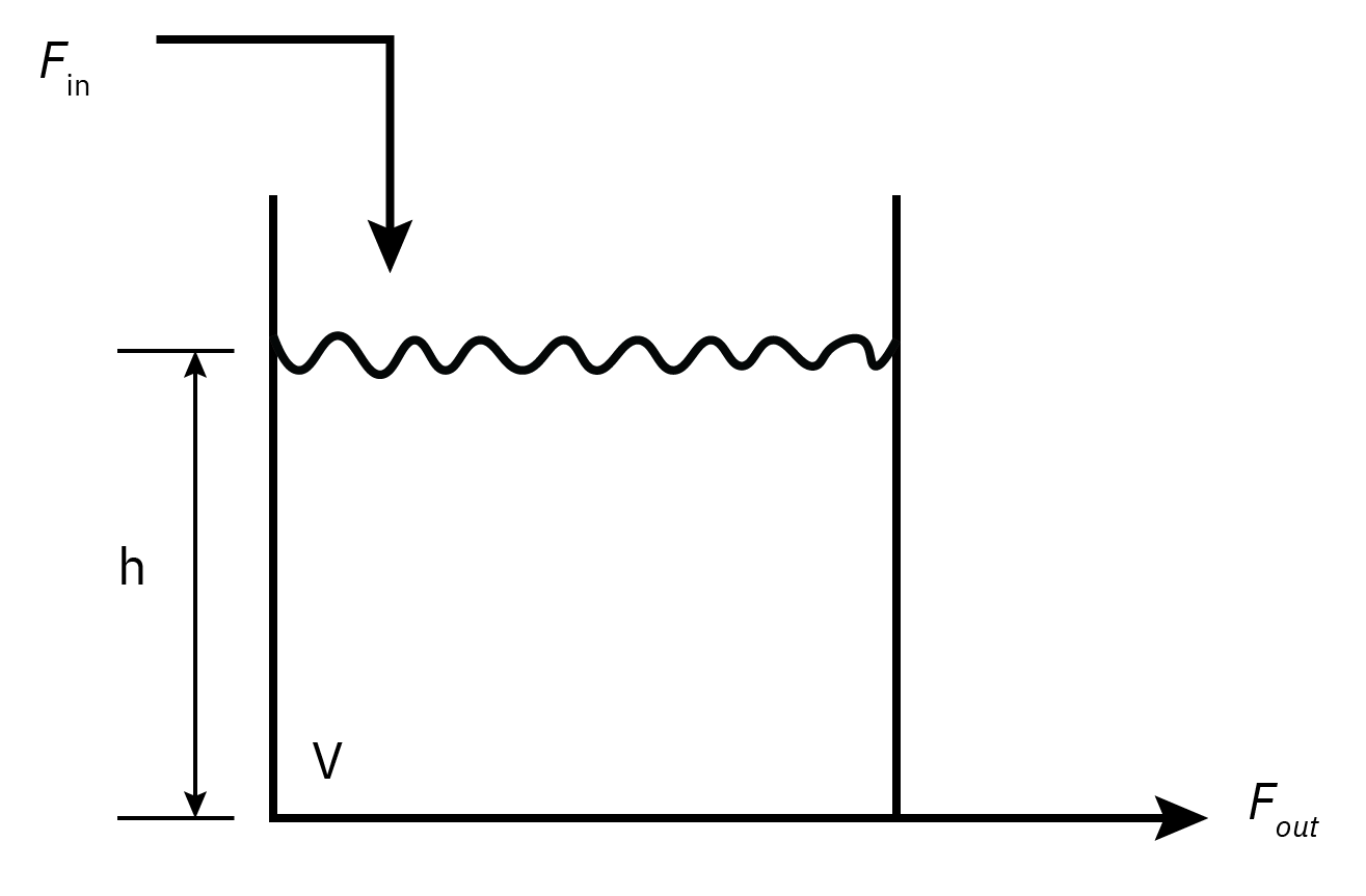
• Manipulated Variable (MV): The flow rate of the liquid into or out of the tank.

• Controlled Variable (CV): Level of the liquid in the tank

• Disturbances: Changes in inlet flow rate, changes in outlet flow rate, temperature variations, pressure fluctuations

• Unmeasured Output: The temperature of the liquid in the tank

Control objectives

Explicit control objectives (ECOs)

• Clearly defined and typically quantifiable goals for the performance of a control system.

• These objectives are explicitly stated

• Form the basis of the formal design and analysis of control systems

• Examples:

  Setpoint Tracking, Disturbance Rejection, Stability, Speed of Response, Overshoot Minimization, Regulatory Compliance

Implicit control objectives (ICOs)

• Not explicitly stated or quantified

• Often evaluated qualitatively

• Have a significant long-term impact

• Play a crucial role in the successful implementation

• Examples:

  Simplicity, Reliability, Cost-effectiveness, Safety, Flexibility, Scalability

Control System Design should link the two types of control objectives.

Real plants can have similar ICOs but different ECOs

Implicit control objectives

Safety First

• People
• Environment
• Equipment

Profit

• meeting final product specifications
• minimizing waste production
• minimizing environmental impact
• minimizing energy use
• maximizing overall production rate

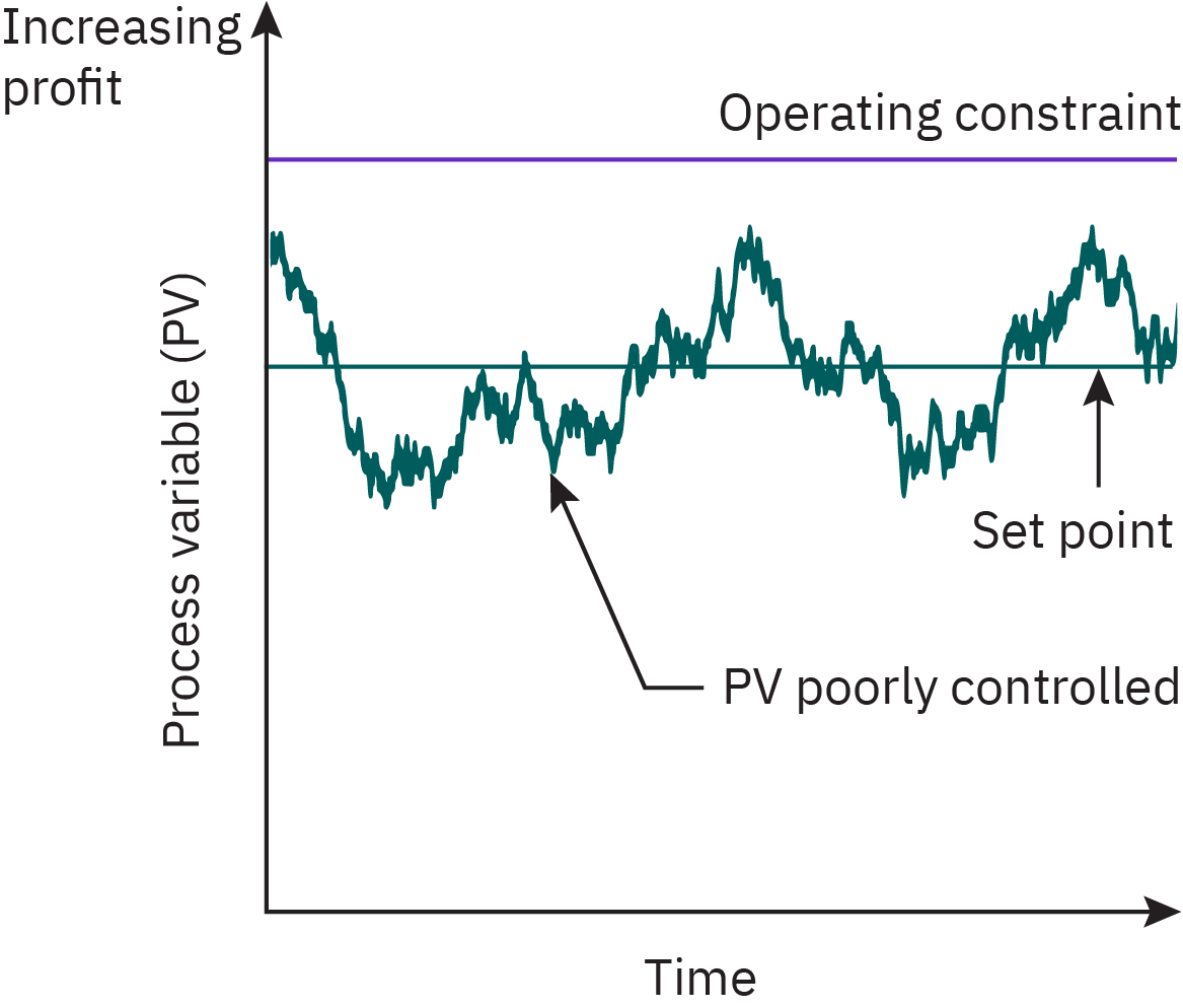
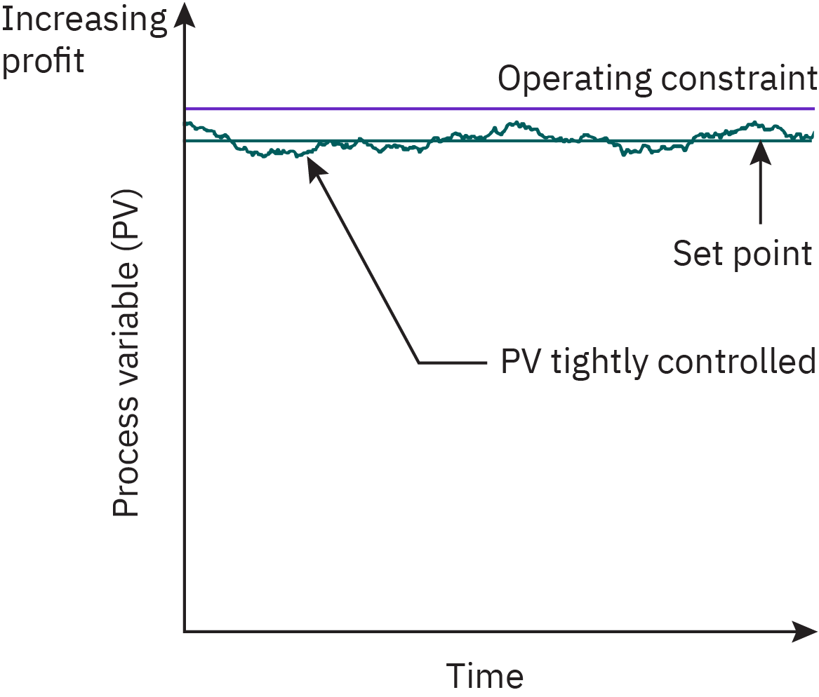
Reducing variability

• Poor control requires set point far from constraint

• Good control permits set point near constraint

Optimal plant operations

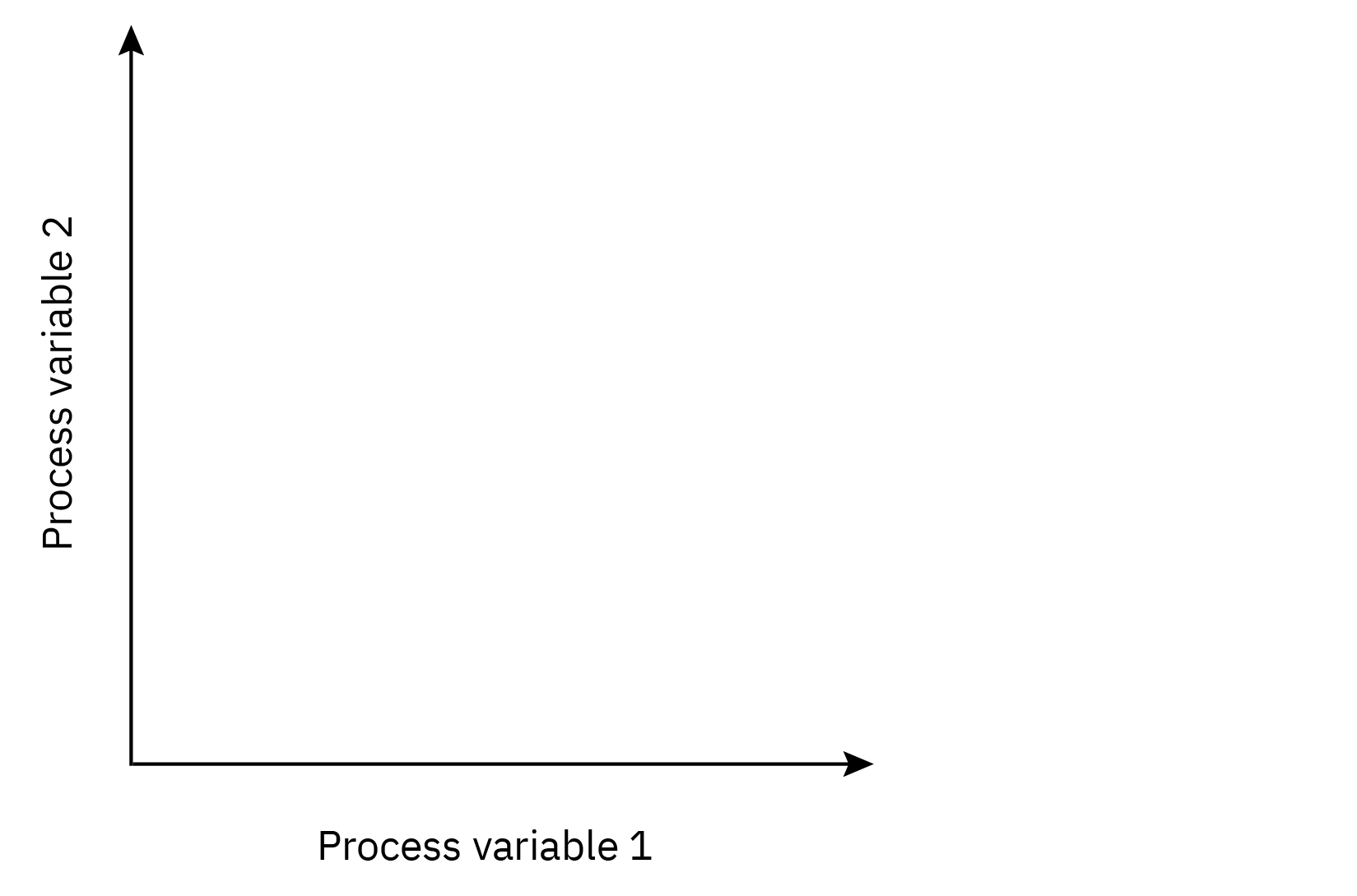
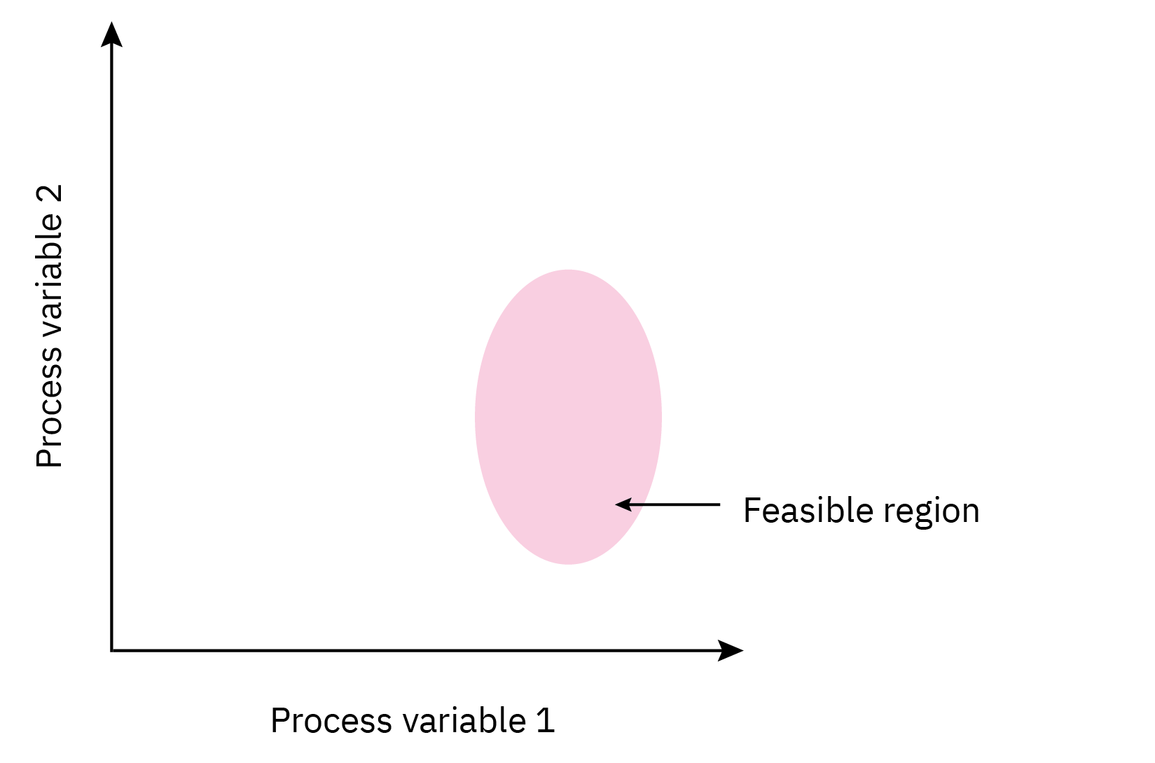
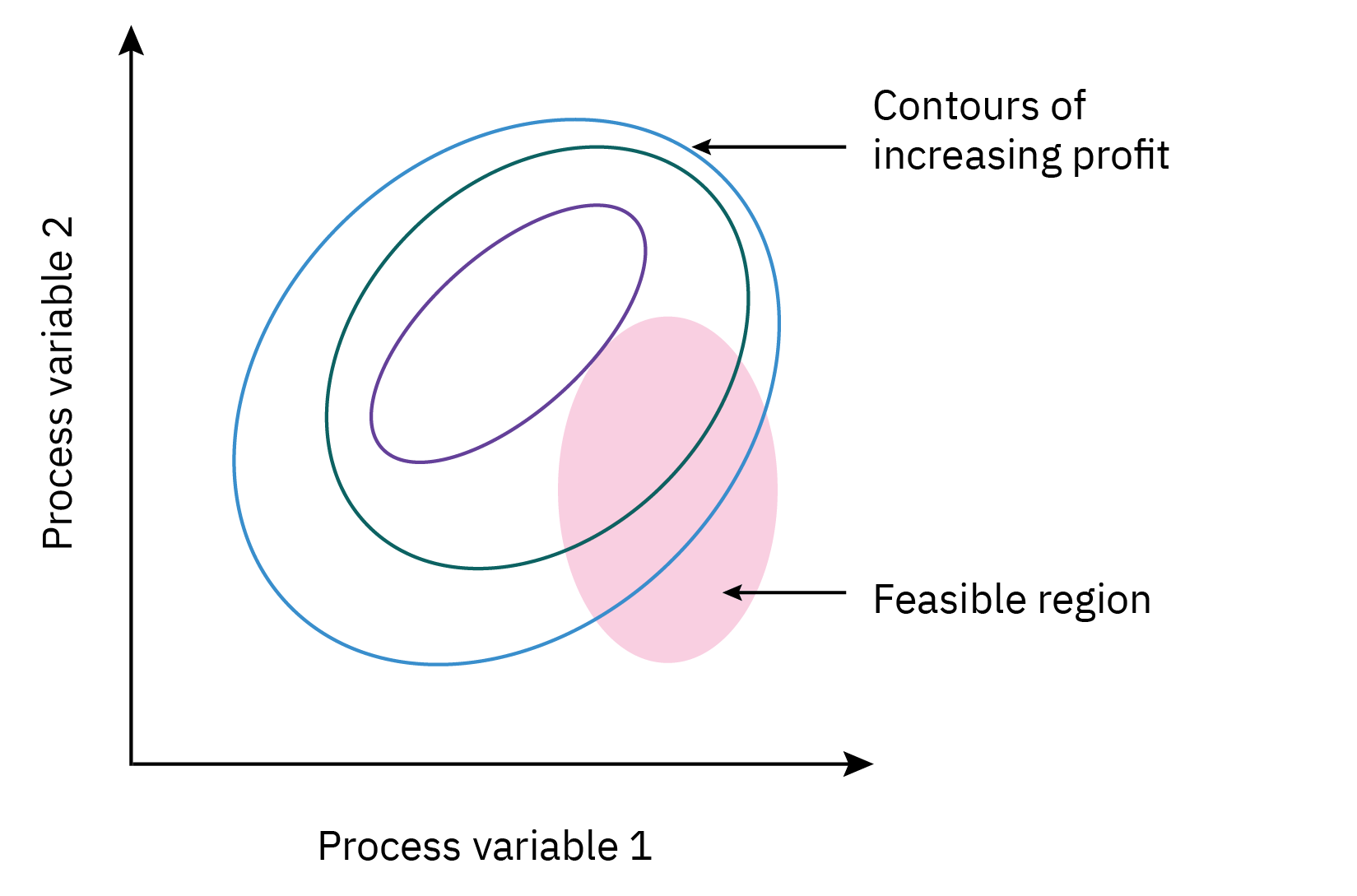
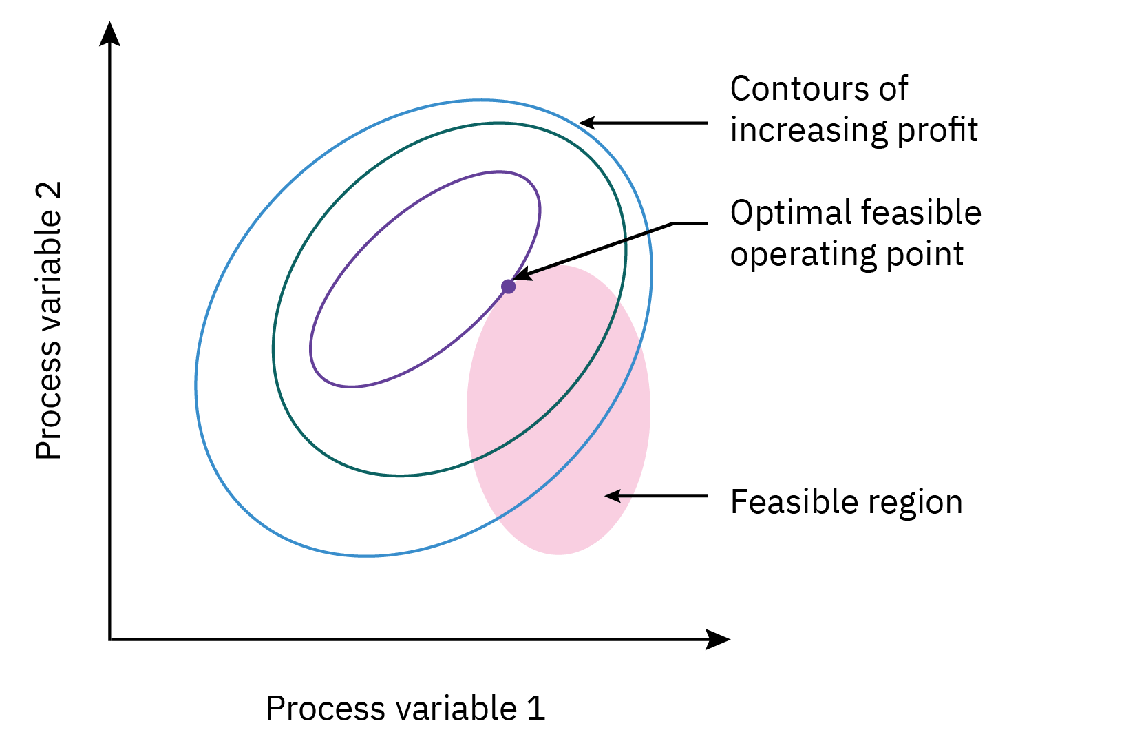
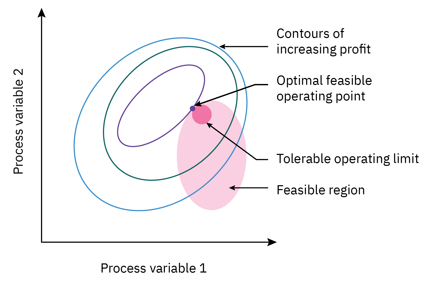
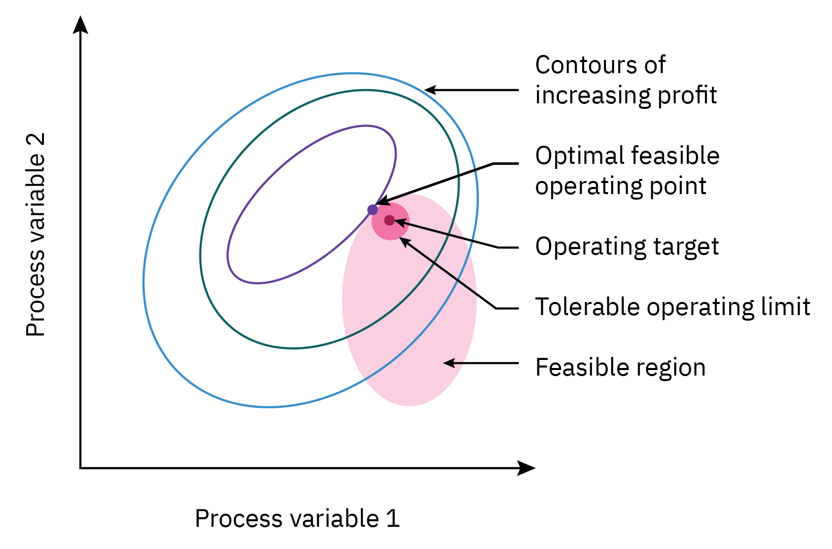
Hirarchy of process control activities

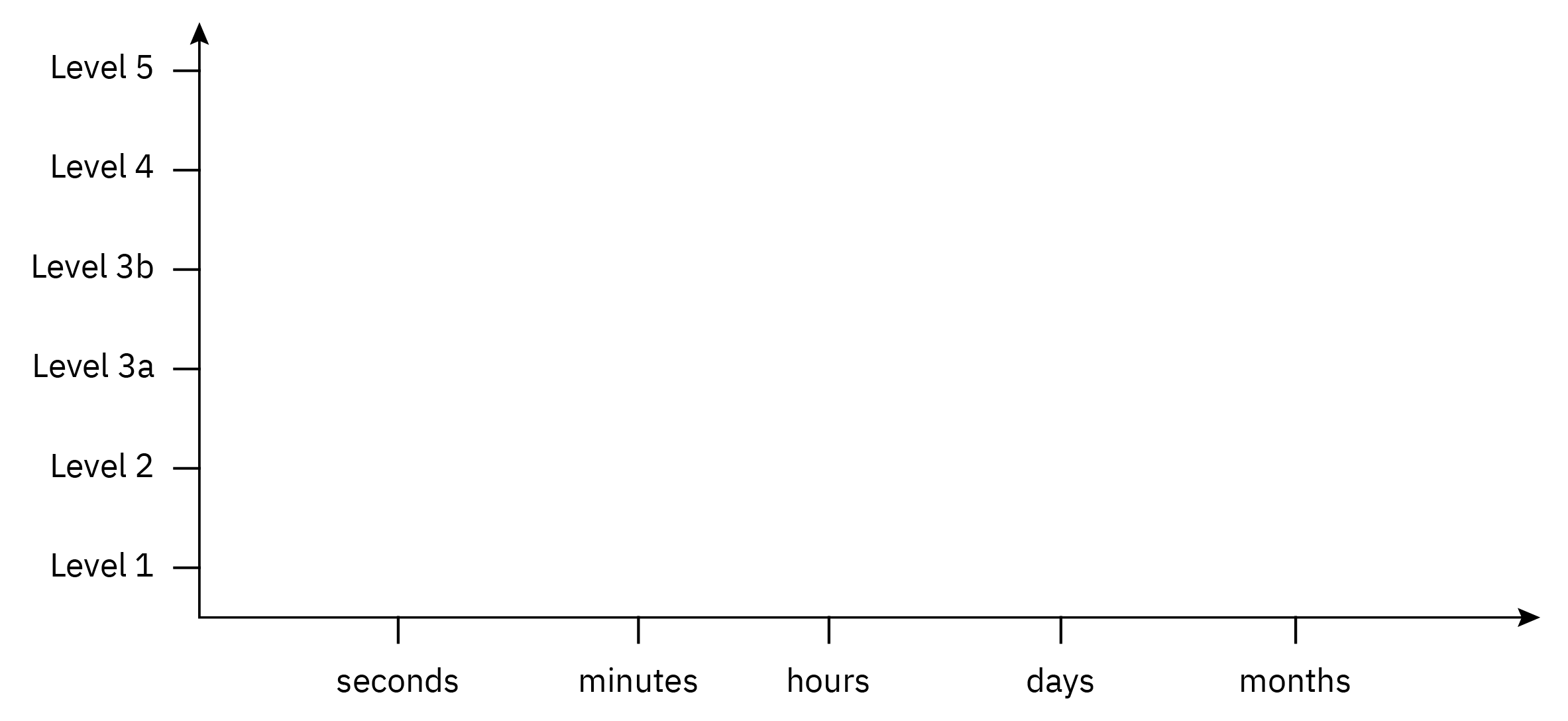
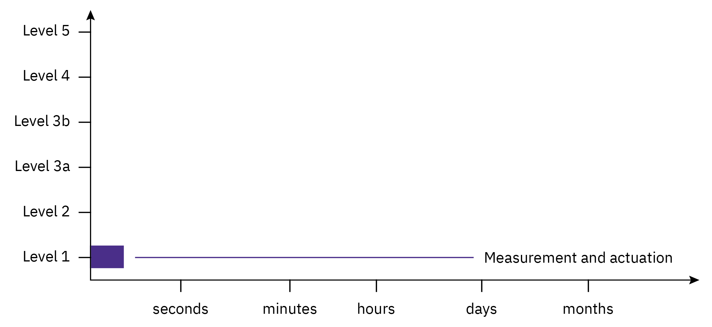
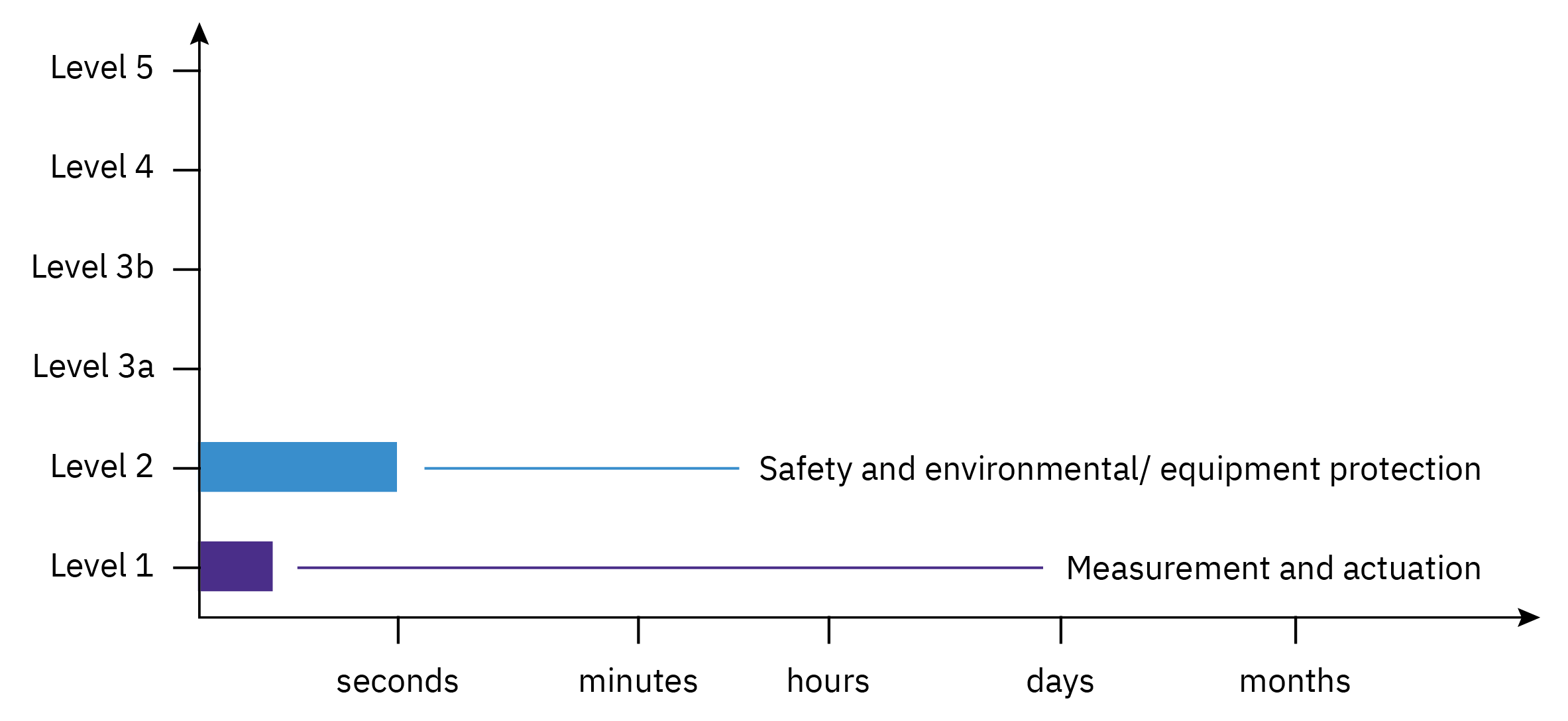
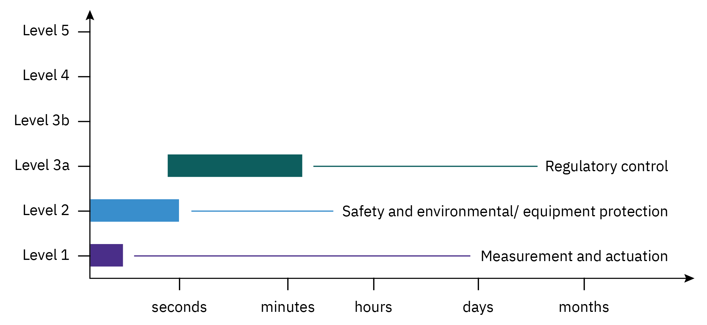
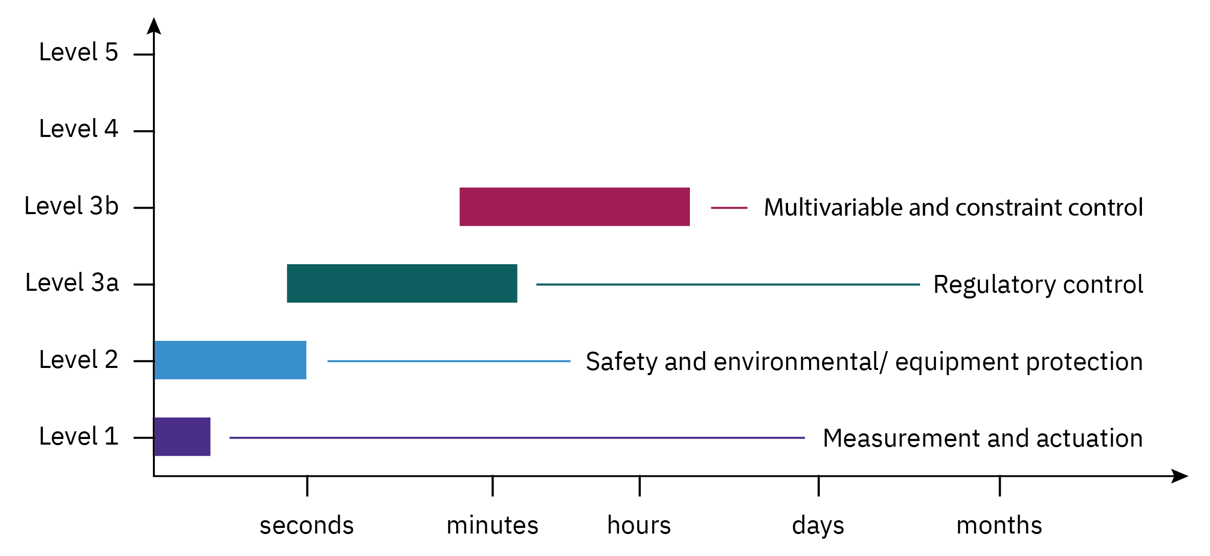
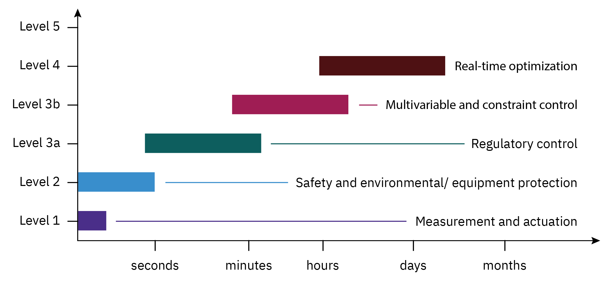
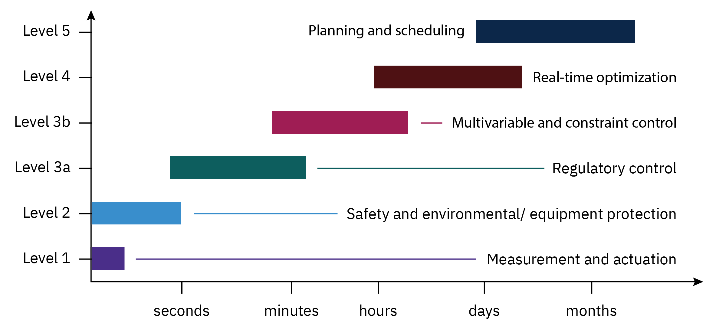
Overview of control system design

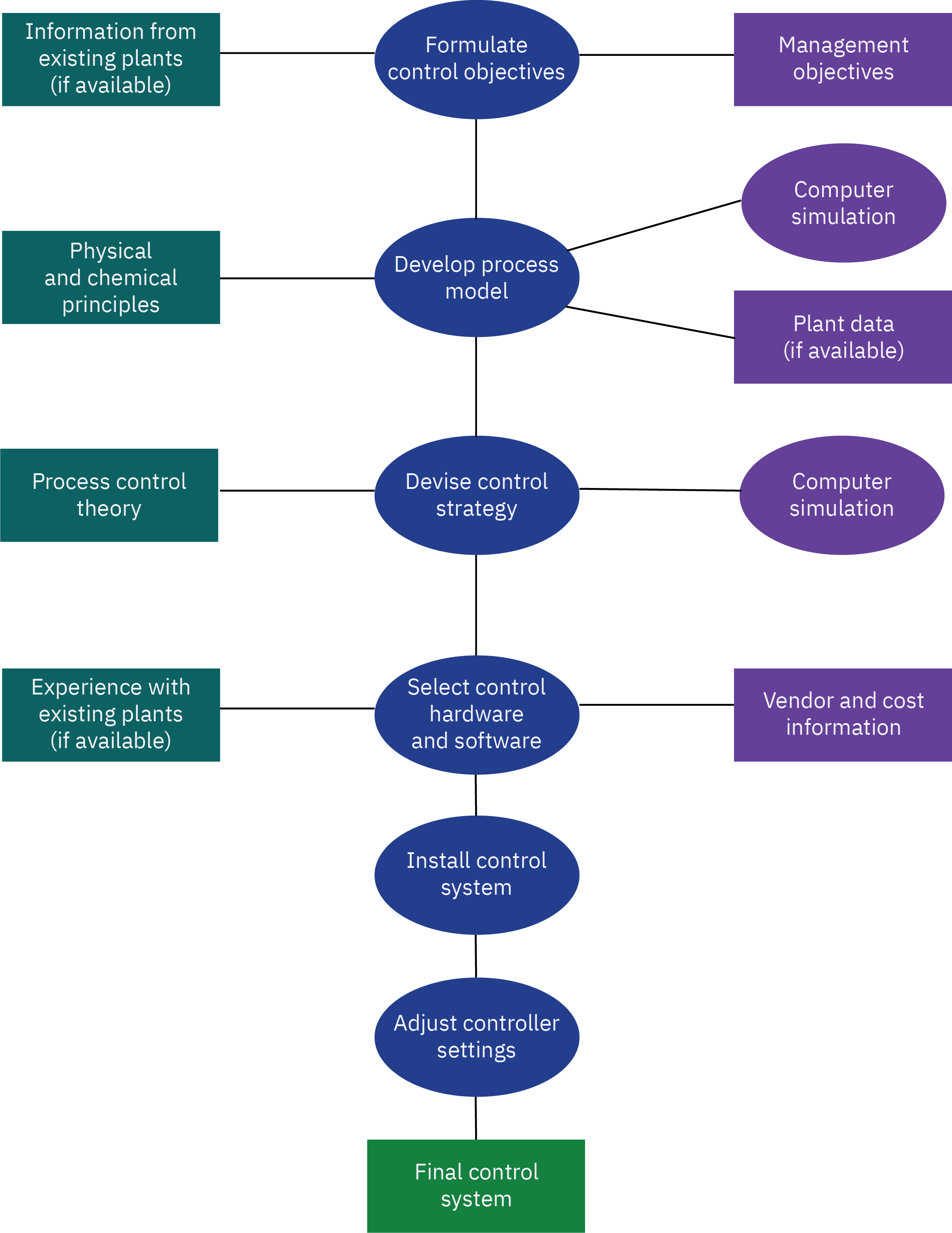
Fundamentals of process modeling

• Why process modeling?
• Types of process models
• Basic principles of mass and energy balances
• Process control terminology

Why process modeling?

• Enhancing Process Understanding

  Enable study of transient behavior without disruption

  Provide valuable insights into dynamic and steady-state process behavior

  Useful even before plant construction

• Process Simulators for Training

  Essential for training plant operators in complex units and emergencies

  Create a realistic training environment when connected to process control equipment

• Facilitating Evaluation of Control Strategies

  Assist in identifying variables to be controlled and manipulated

  Aid in preliminary controller tuning

  Play an explicit role in model-based control strategies

• Optimization of Operating Conditions

  Recalculation of optimum conditions maximizes profit or minimizes costs

  Utilize steady-state process model and economic data

  Allow for continuous enhancement of process performance

Types of process models

• Theoretical models

  Developed using the principles of chemistry, physics, and biology.

  First principles models

  Mass, momentum, and heat balances

• Empirical models

  Obtained by fitting experimental data.

  Statistical models

  Correlations

  data driven models

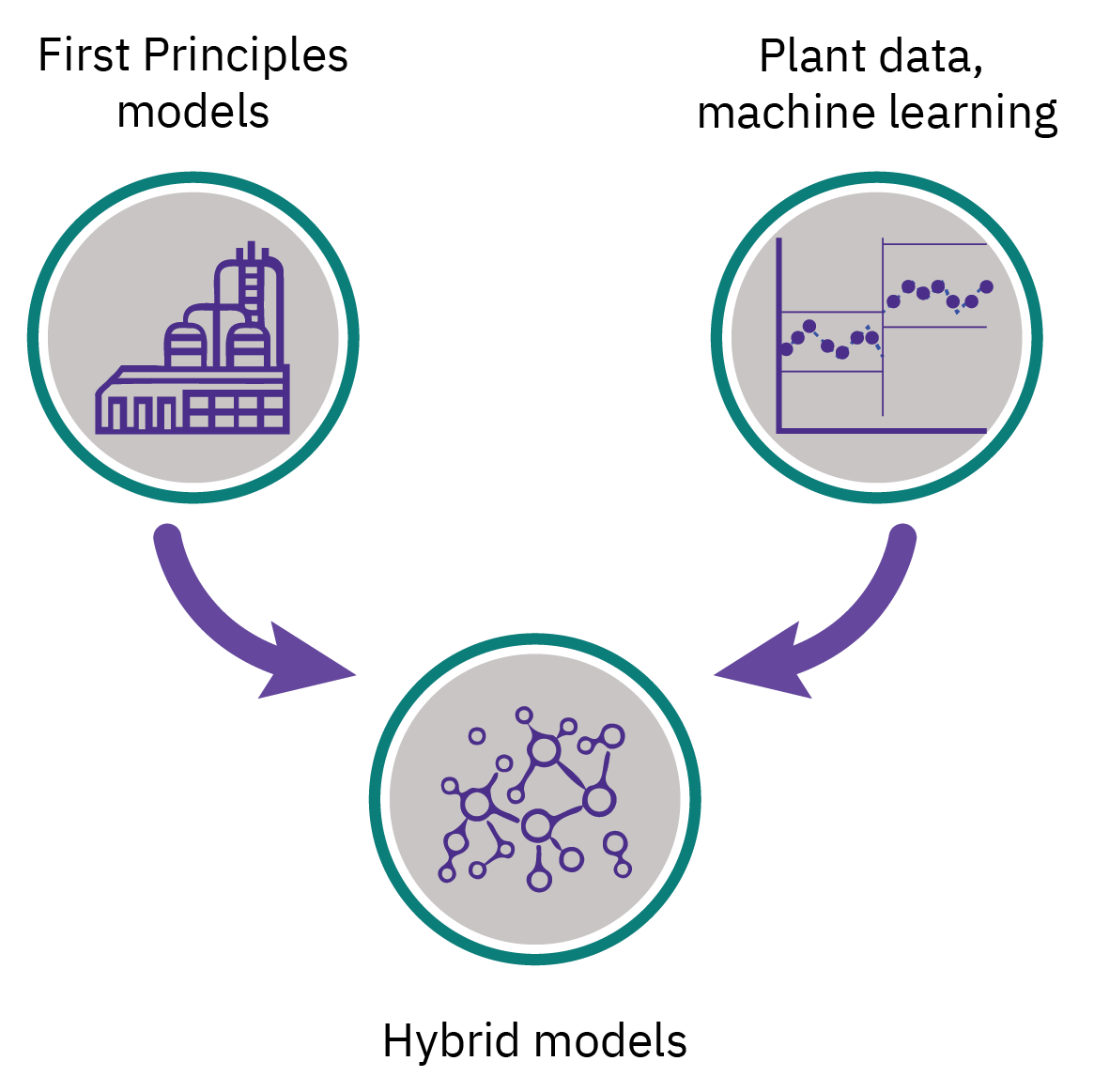
• Semi-empirical/ hybrid models

  A combination of the theoretical and empirical models

  The numerical values of one or more of the parameters in a theoretical model are calculated from experimental data.

Basic principles of mass and energy balances

• In general

  \text{accumulation} = \text{in} - \text{out} - \text{reaction} - \text{tranfer}

• Mass balance (without reaction and transfer)

  \left\{\begin{array}{c} \text {rate of mass} \\ \text {accumulation} \end{array}\right\} = \left\{\begin{array}{c} \text {rate of} \\ \text {mass in} \end{array}\right\} - \left\{\begin{array}{c} \text {rate of} \\ \text {mass out} \end{array}\right\}

• For component i (with reaction term included)

  \left\{\begin{array}{c} \text {rate of} \\ \text {component i} \\ \text {accumulation} \end{array}\right\} = \left\{\begin{array}{c} \text {rate of} \\ \text {component i} \\ \text {in} \end{array}\right\} - \left\{\begin{array}{c} \text {rate of} \\ \text {componenti } \\ \text {out} \end{array}\right\} + \left\{\begin{array}{c} \text {rate of} \\ \text {component i} \\ \text {produced} \end{array}\right\}

Basic principles of mass and energy balances

• Energy balance

\begin{aligned} \left\{\begin{array}{c} \text { rate of energy } \\ \text { accumulation } \end{array}\right\} &= \left\{\begin{array}{c} \text { rate of energy in } \\ \text { by convection } \end{array}\right\} \\ & -\left\{\begin{array}{c} \text { rate of energy out } \\ \text { by convection } \end{array}\right\} \\ & +\left\{\begin{array}{c} \text { net rate of heat addition } \\ \text { to the system from } \\ \text { the surroundings } \end{array}\right\} \\ & +\left\{\begin{array}{c} \text { net rate of work } \\ \text { performed on the system } \\ \text { by the surroundings } \end{array}\right\} \end{aligned}

Blending of two components

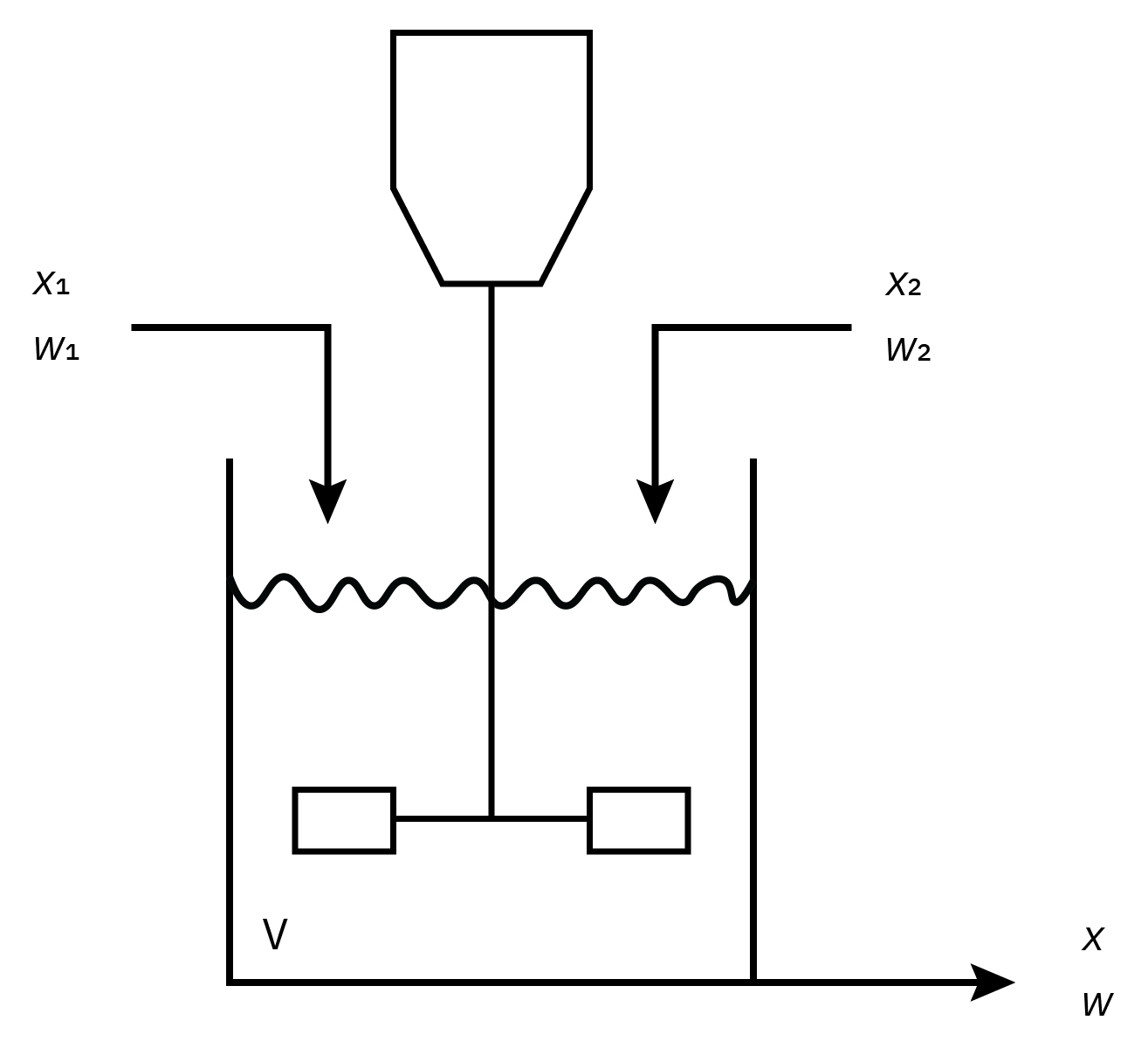
• Overall mass balance

  \left\{\begin{array}{c} \text {rate of accumulation} \\ \text {of mass in the tank} \end{array}\right\} = \left\{\begin{array}{c} \text {rate of} \\ \text {mass in} \end{array}\right\} - \left\{\begin{array}{c} \text {rate of} \\ \text {mass out} \end{array}\right\}

  \frac{d(V \rho)}{dt} = w_1 + w_2 - w

• Component balance

  \frac{d(V \rho x)}{dt} = w_1 x_1 + w_2 x_2 - w x

Blending of two components

• Overall mass balance

  \left\{\begin{array}{c} \text {rate of accumulation} \\ \text {of mass in the tank} \end{array}\right\} = \left\{\begin{array}{c} \text {rate of} \\ \text {mass in} \end{array}\right\} - \left\{\begin{array}{c} \text {rate of} \\ \text {mass out} \end{array}\right\}

  \frac{d(V \rho)}{dt} = w_1 + w_2 - w

• Component balance

  \frac{d(V \rho x)}{dt} = w_1 x_1 + w_2 x_2 - w x

It is possible to further simplify the system of two differential equations to

\frac{dV}{dt} = \frac{1}{\rho}\left(w_1 + w_2 - w \right)

\frac{dx}{dt} = \frac{w_1}{V \rho} \left(x_1 - x\right)+ \frac{w_2}{V \rho} \left(x_2 - x\right)

Degrees of freedom analysis

• To simulate a process, it’s crucial to confirm that the model equations, both differential and algebraic, form a set of relations that can be solved.

• For the model to have a unique solution, the number of unknown variables should match the number of independent model equations.

• N_F = N_V - N_E

  1. N_F = 0: The process model is exactly specified. If NF = 0, then the number of equations is equal to the number of process variables and the set of equations has a solution. (However, the solution may not be unique for a set of nonlinear equations.)

  2. N_F > 0: The process is underspecified. If N_F > 0, then N_V > N_E, so there are more process variables than equations. Consequently, the N_E equations have an infinite number of solutions, because NF process variables can be specified arbitrarily.

  3. N_F < 0: The process model is overspecified. For N_F < 0, there are fewer process variables than equations, and consequently the set of equations has no solution.

Solution of model equations

• Nonlinear Chemical Processes: These result in complex ordinary differential equations when modeled.

• Linear System Controls: These tools are well-established and provide valuable insights when processes operate near a specific point.

• Laplace Transform: This simplifies creation of input-output models by converting differential equations to algebraic ones.

• Transfer Function: An essential tool in control system design and analysis, representing linear control theory.

Empirical models

• We can construct an empirical model using plant data

• Assume a certain idealized model structure

• First-order plus deadtime (FOPDT) model

  Time domain form \tau_p \frac{dy(t)}{dt} + y(t) = K_p u(t - \theta_p)

  Frequency domain form (transfer function) G_p(s) = \frac{K_p e^{-\theta_p s}}{\tau_p s + 1}

• K_p: Process gain; \tau_p: time constant; \theta_p: deadtime

FOPDT model is often used in controller tuning. A transfer function is a mathematical formula that describes how a system responds to different inputs over time.

Second-Order plus Deadtime (SOPDT) Model

• Time domain

  \tau^2 \frac{ d^2 y(t)}{dt^2} + 2 \xi \tau \frac{d y(t)}{dt} + y(t) = K_p u(t - \theta)

• Frequency domain

  G_p(s) = \frac{Y(s)}{U(s)} = \frac{K_p e^{-\theta s}}{\tau^2 s^2 + 2 \xi \tau s + 1}

• K_p: Process gain; \tau: time constant; θ: dead time; \xi: damping factor or coefficient

• Behavior:

  \xi > 1: Overdamped

  0 < \xi < 1: Underdamped

  \xi = 1: Critically damped

  \xi = 0: Sustained oscillations

  \xi < 0: Unstable

Dynamic Behavior of Processes

• Input types
• Response of first-order systems
• Response of second-order systems
• Properties of transfer functions
• Stability of linear systems

Input types

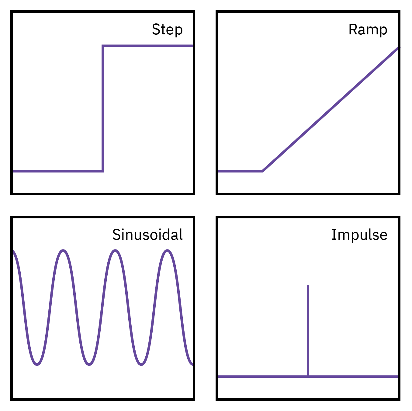
Response of first-order systems

• Overall mass balance

  A \frac{dh}{dt} = F_{in} - F_{out}

• Outlet flow rate, F_out has a square-root dependence on liquid level F_{out} = \beta \sqrt{h}

• Resulting nonlinear equation

  A \frac{dh}{dt} = F_{in} - \beta \sqrt{h}

  \tau \frac{d \bar{h}}{dt} + \bar{h} = kF_{in} ; \, \tau = \frac{2A\sqrt{h}}{\beta} ; \, k = \frac{2 \sqrt{h}}{\beta}

• Transfer function

  \frac{\bar{h}(s)}{\bar{F_in}(s)} = g(s) = \frac{k}{\tau s + 1}

• Process gain (k): Ultimate value of the response (new steady-state) for a unit-step change in the input.

• Time constant (τ): Time necessary for the process to adjust to a change in the input.

Response of first-order systems

• The ultimate (steady-state) value of the response, \bar{h} (t \to \infty), is equal to k for a unit-step change.

• When the elapsed time is equal to the process time constant t = \tau, the system reaches 63.2% of its final response.

• After approximately 5τ, the transient response can be considered as having reached steady-state.

• For a given t / τ, the output reaches the same fraction of the ultimate output response value.

In a tank process, a rise in the inlet flow rate elevates the liquid level, which in turn increases the hydrostatic pressure and subsequently the outlet flow rate. The system eventually reaches a new steady state. This feature is termed ‘self-regulation’.

Response of first-order systems

Response of second-order systems

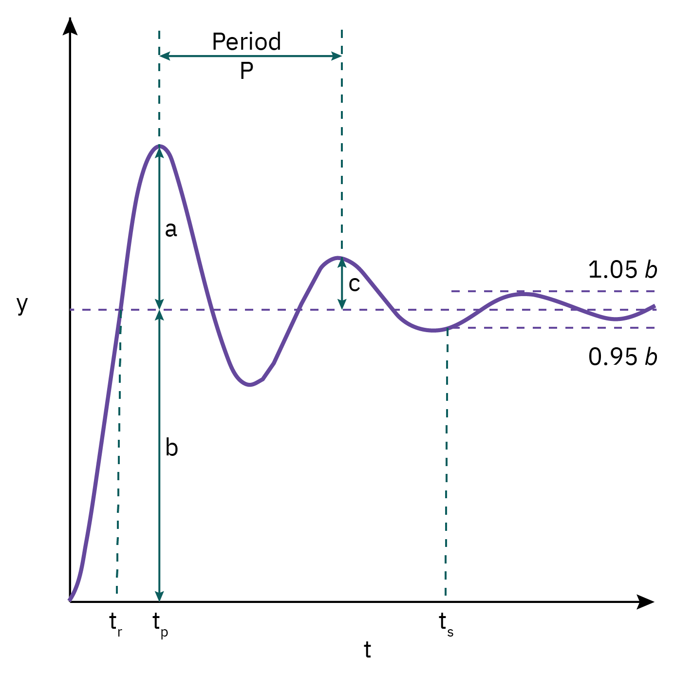
• Rise time (t_r): time required for y(t) to first cross its new steady state value

• Overshoot (a/b): The maximum amount by which the response exceeds the new steady state value

• Decay ratio (c/a): Ratio of the height of successive peaks in the response

• Period of oscillation (P): time for a complete cycle

• Response/ settling time (t_s): time required for the response to remain within a ± 5% band based upon steady state value.

Decay ratio, overshoot, response time, and damping factor (ξ) can be used as a basis for tuning.

Response of second-order systems

Critically damped (ξ = 1)

• Output response becomes more sluggish as τ increases.

• The responses are qualitatively similar.

Effect of ξ

• ξ < 1: Oscillation and overshoot

• ξ > 1: Sluggish response, no oscillations; no overshoot

• ξ = 1: Fastest response, no oscillations; no overshoot

Properties of transfer functions

• For transfer function

  g(s)= \frac{y(s)}{u(s)} = \frac{b_0 s^m + \ldots + b_m}{a_0 s^n + \ldots + a_n} = \frac{z(s)}{p(s)}

• The roots of the polynomial z(s) are the zeros of the transfer function or the zeros of the process.

• The roots of the polynomial p(s) are the poles of the transfer function or the poles of the process.

• A physical system needs to be proper (n \geq m), and casual (output depends only on past inputs)

• Characteristic equation

  The denominator polynomial p(s) when equated to zero is called the characteristic equation:

  p(s) = a_0 s^n + \ldots + a_n = 0

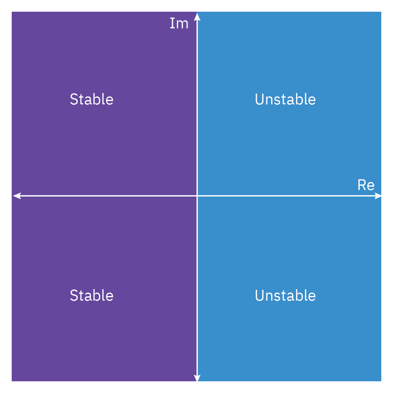
Stability of linear systems

• The location of the poles of a transfer function determines the bounded input–bounded output (BIBO) stability of a process.

• If the transfer function of a dynamic process has a pole with a positive real part, the process is unstable. If the real part is zero, then the process is critically stable

• We need to be cautious when we derive a transfer function model from a statespace model, because a zero (or zeros) may cancel a pole (or poles). This becomes especially important if the canceled pole is unstable, which means that those modes of the process would be hidden from us.

Routh’s Stability Criterion

Routh’s Criterion is a mathematical test that is used to determine whether a linear system is stable or unstable. It does not require explicit calculation of the roots of the characteristic equation.

• The first step in Routh’s Criterion is to set up the Routh array.

• Then, we examine the first column of the array. If there are no sign changes in the first column, the system is stable.

• If there are sign changes in the first column, the system is unstable. The number of sign changes corresponds to the number of roots with positive real parts.

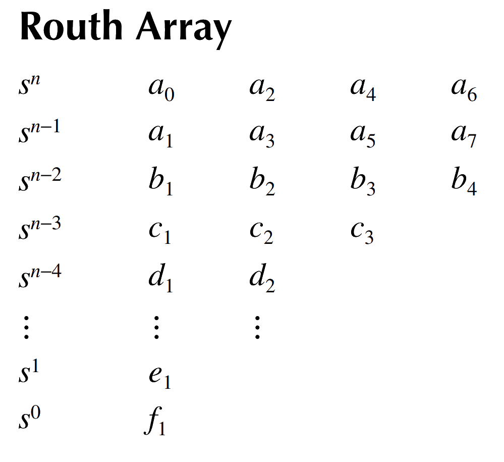
Routh’s Criterion can also be used to determine relative stability and system type.

Root locus method

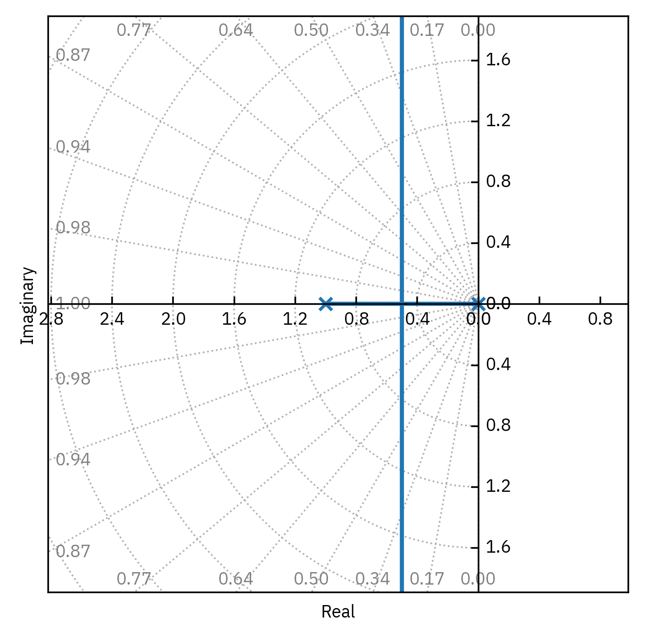
Root Locus is a graphical method used in control systems to examine how the system stability changes with varying gain.

• It shows possible pole locations as system gain varies from zero to infinity.

• The method provides insights into stability and transient response.

• Root locus begins at open-loop poles and ends at open-loop zeros.

• The plot exists on parts of the complex plane where the number of open-loop poles and zeros to the right is odd.

• Consider the characteristic equation p(s,k)= s^2 + s + k =0

Feedback Control Systems

• Introduction to feedback control
• Control law
• Proportional, integral, and derivative control actions
• Further topics

Introduction to feedback control

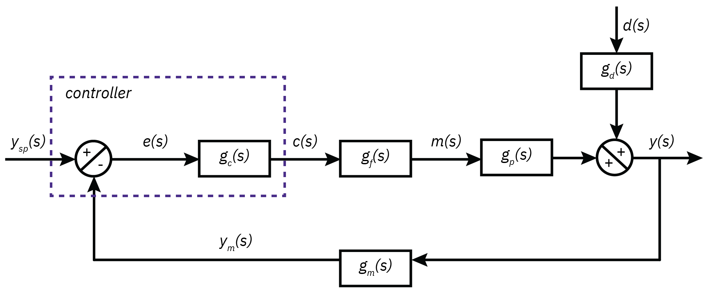
Introduction to feedback control

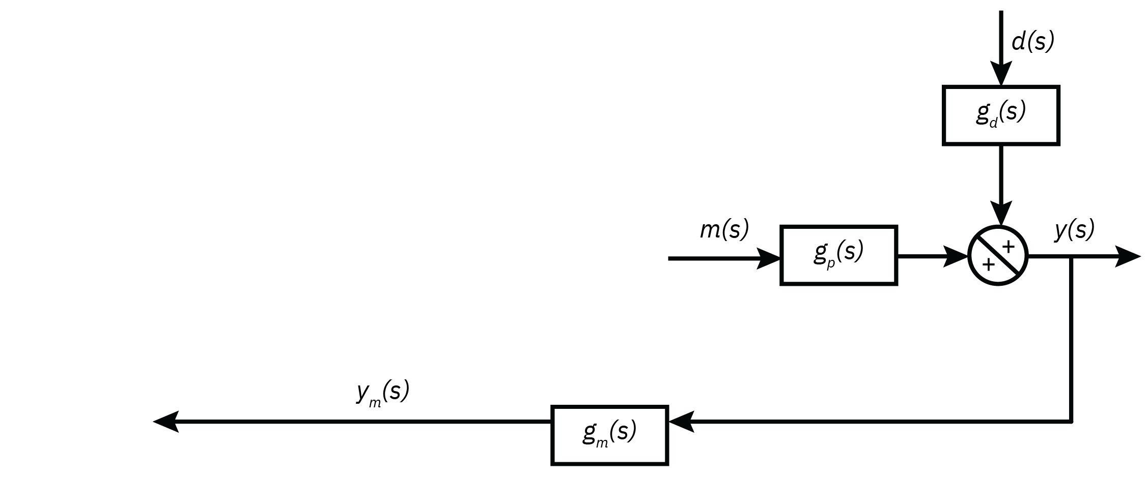
• y = g_p m + g_d d

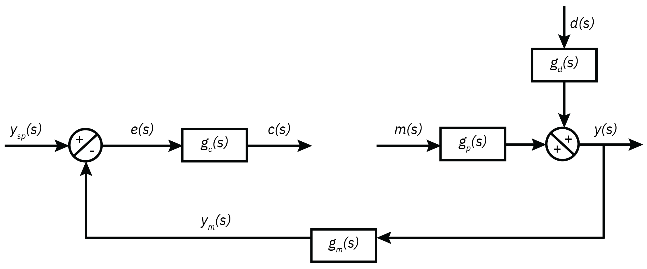
• Error: e = y_{sp} - y_m

• Control action: c = g_c e = g_c(y_{sp} - y_m)

• Manipulated variable: m = g_f c = g_c g_f (y_{sp} - y_m)

• Controlled variable: y = g_p m + g_d d = g_c g_f g_p (y_{sp} - y_m) + g_d d

• Closed loop transfer function y = \frac{g_p g_f g_c}{1 + g_p g_f g_c g_m} y_{sp} + \frac{g_d}{1 + g_p g_f g_c g_m} d

Introduction to feedback control

y = G_{sp} y_{sp} + G_d d

• G_{sp} embodies the dynamics of the setpoint response.
  How the process output will respond when the set-point is changed?

• G_d(s) indicates how the process output will respond when a disturbance enters the process.

• Denominators of the closed-loop transfer functions, G_{sp} and G_{d}, are the same, indicating that they share the same stability characteristics.

• In a more general setting, the closed-loop transfer function for general block diagram is represented as

  \frac{r(s)}{r_i(s)} = \frac{G_1(s)}{1 + G_2(s)}

  In this expression, r is an output variable or any internal variable within the control loop and r_i represents an input variable such as y_{sp} or d.

  The transfer function G_1 is the product of the transfer functions in the forward path that connects an input r_i to an output r.

  G_2 is the transfer function composed of all transfer functions in the feedback loop.

Introduction to feedback control

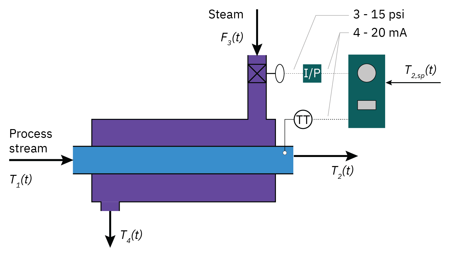
Introduction to feedback control

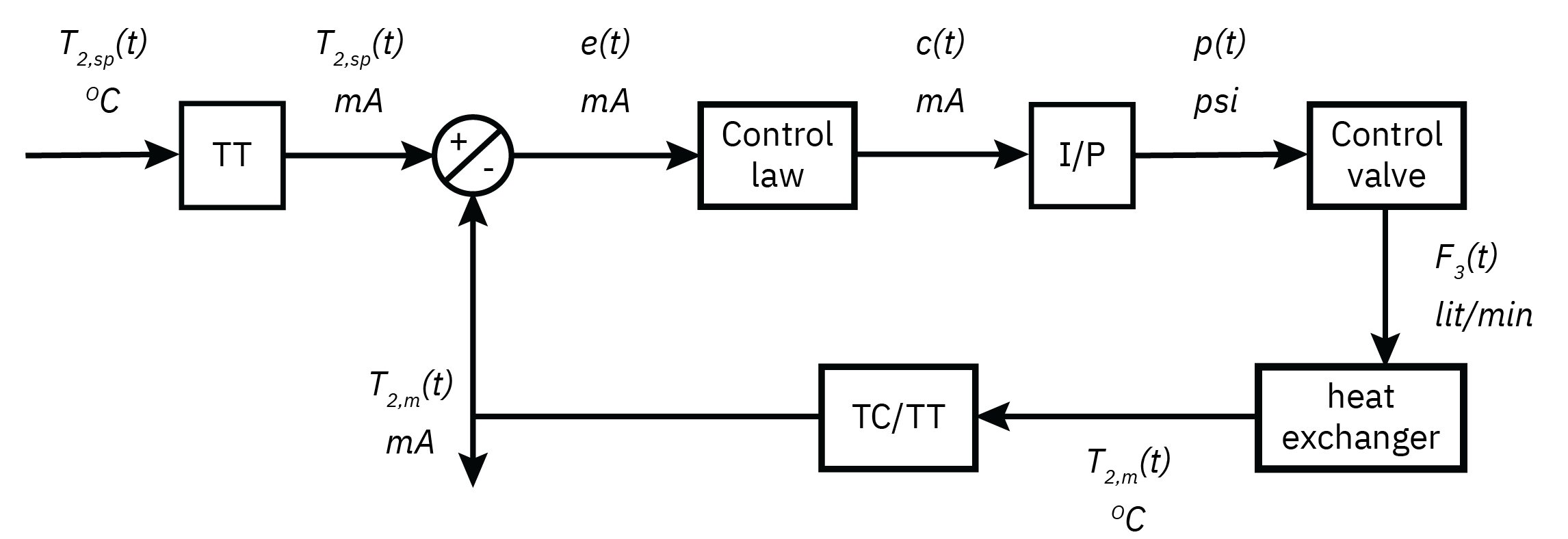
Control law

• The control signal c(t) is calculated, given the value of the error e(t), through a predefined functional relationship c(t) = C \left[e(t)\right]

• The function C[\cdot] constitutes teh control law.

• Establishes the manner with which the error information is processed by the controller.

• The most common functional form is the three-mode proportional–integral– derivative (PID) control law \frac{\bar{c}(s)}{\bar{e}(s)} = g_c(s) = k_c \left(1 + \frac{1}{\tau_I s} +\tau_D s \right)

Proportional mode

• This mode produces a control signal that is proportional to the error: c(t) = k_c e(t) + c_b

• k_c represents the proportional gain of the controller: Defines how sensitive the controller is to errors present in the system.

• c_b is a bias signal that corresponds to the value of the control signal when the error is zero. The bias signal is the steady-state value of the control signal.

• Define - deviation variable \bar{c}(t) = c(t) - c_b; also \bar{e}(t) = e(t)

• Transfer function: \frac{\bar{c}(s)}{\bar{e}(s)} = g_c(s) = k_c

Proportional mode

Integral mode

• The control signal for this mode is produced by the integral equation: c(t) = \frac{k_c}{\tau_I}\int{e(t)dt} + c_b

• The new parameter \tau_I represents the integral time constant or the reset time.

• With this mode, the controller responds effectively to errors that build up over time.

  This is a very important feature because even if the error is small, as long as it persists, a large control signal may be calculated, thus helping to eliminate the error quickly

• The transfer function of a controller with only the integral mode is \frac{\bar{c}(s)}{\bar{e}(s)} = g_c(s) = k_c \left(\frac{1}{\tau_I s} \right)

Integral mode

Derivative mode

• In this mode, the control signal responds to the rate of change of the error signal: c(t)= k_c \tau_D \frac{\mathrm{d}e(t)}{\mathrm{d}t} + c_b

• A new parameter \tau_D is introduced as the derivative time constant.

• The role of this mode is to judge the change in the error.

  For instance, if the error is still present but not increasing as fast, the controller may use this information to decrease the control signal, thus possibly avoiding overly aggressive control actions.

• The transfer function for a controller with derivative mode only is given by \frac{\bar{c}(s)}{\bar{e}(s)} = g_c(s) = k_c \left(\tau_D s \right)

Derivative mode

Mixing tank

• The manipulated variable is the flow rate of stream 2, F_2, to control the outlet mass fraction, x.

• The disturbance is the flow rate of stream 1, F_1.

• The feed mass fractions are assumed constant.

• There is a P controller, g_c(s) = k_c.

• The dynamics of the actuators and the sensors are accounted for by pure dead-time elements, resulting in the transfer functions

  \bar{x}(s) = \frac{-0.1 e^{-s}}{2.5s + 1} \bar{F}_1(s) + \frac{ 0.1 e^{-s}}{2.5s + 1} \bar{F}_2(s)

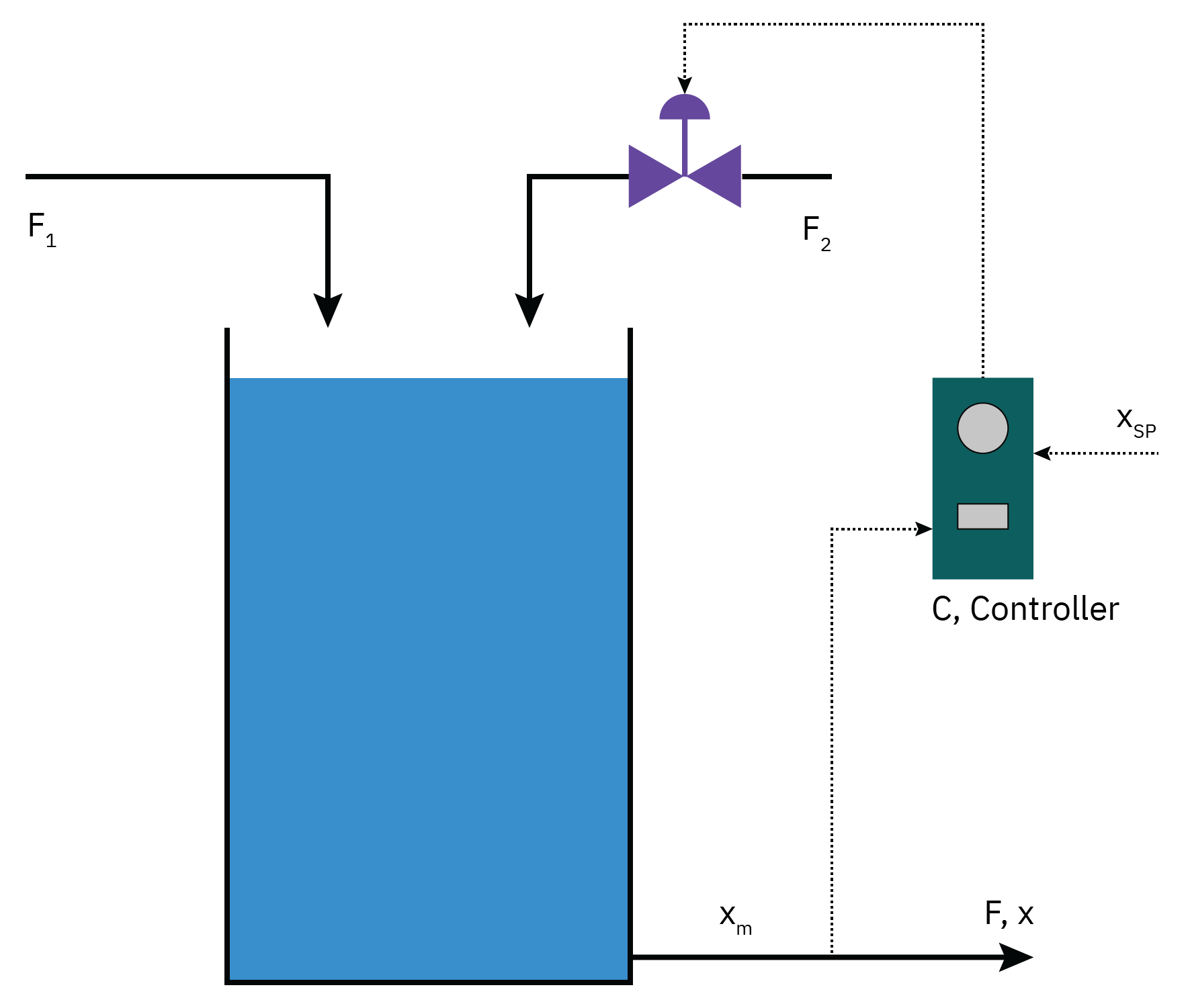
Mixing tank: setpoint change

Mixing tank: disturbance rejection

Further topics

• Model liniarization

• Controller design and tuning methods

• Frequency response analysis

• Bode plots and Nyquist plots