Recap: Basics of Process Control and Modelling
Advanced Modeling and Control
Importance of process analysis and control


- Optimal process operations require efficient and effective control
- Control systems and advanced algorithms are deployed to monitor, regulate, and optimize the process variables.
Process System, Input and Output


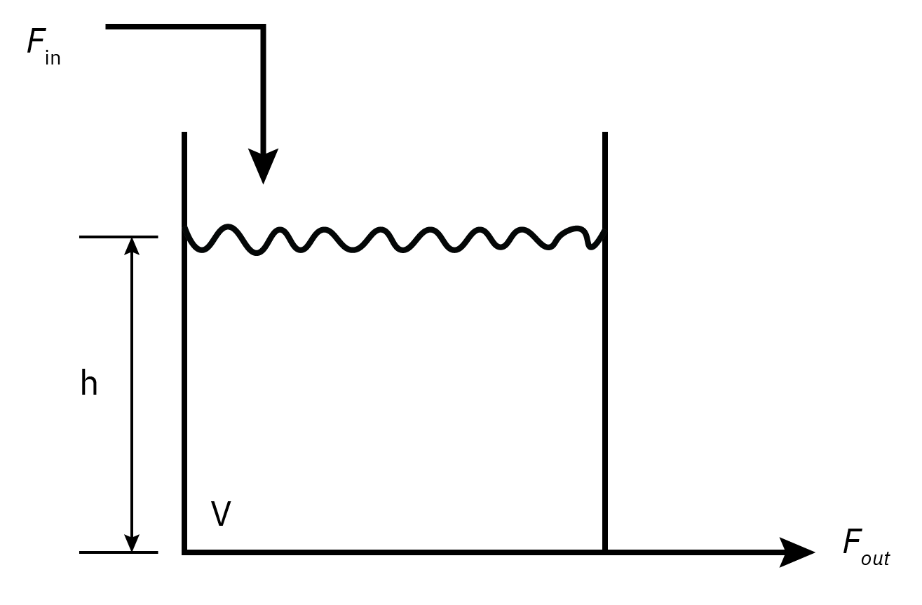
Manipulated Variable (MV): The flow rate of the liquid into or out of the tank.
Controlled Variable (CV): Level of the liquid in the tank
Disturbances: Changes in inlet flow rate, changes in outlet flow rate, temperature variations, pressure fluctuations
Unmeasured Output: The temperature of the liquid in the tank
Implicit control objectives
Safety First
- People
- Environment
- Equipment
Profit
- meeting final product specifications
- minimizing waste production
- minimizing environmental impact
- minimizing energy use
- maximizing overall production rate
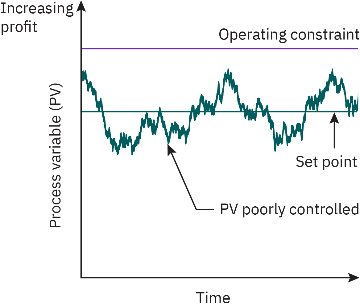
Reducing variability
Poor control requires set point far from constraint
![]()
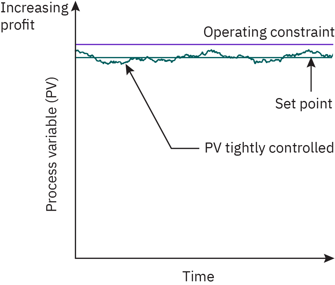
Good control permits set point near constraint
![]()
Optimal plant operations


Hirarchy of process control activities


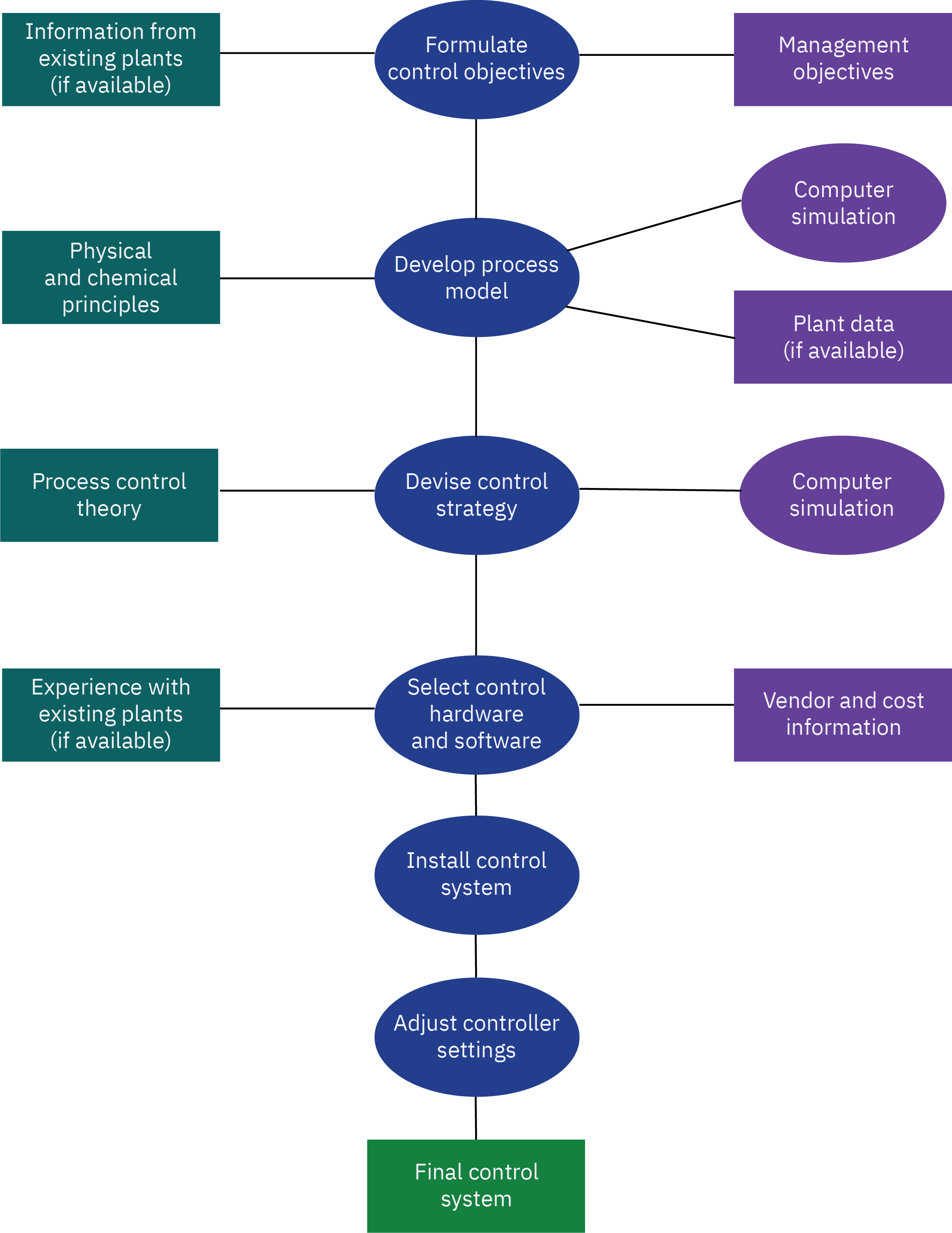
Overview of control system design
Types of process models
Theoretical models
Developed using the principles of chemistry, physics, and biology.
First principles models
Mass, momentum, and heat balances
Empirical models
Obtained by fitting experimental data.
Statistical models
Correlations
data driven models
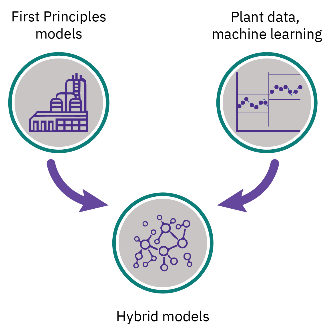
Semi-empirical/ hybrid models
A combination of the theoretical and empirical models
The numerical values of one or more of the parameters in a theoretical model are calculated from experimental data.
Blending of two components
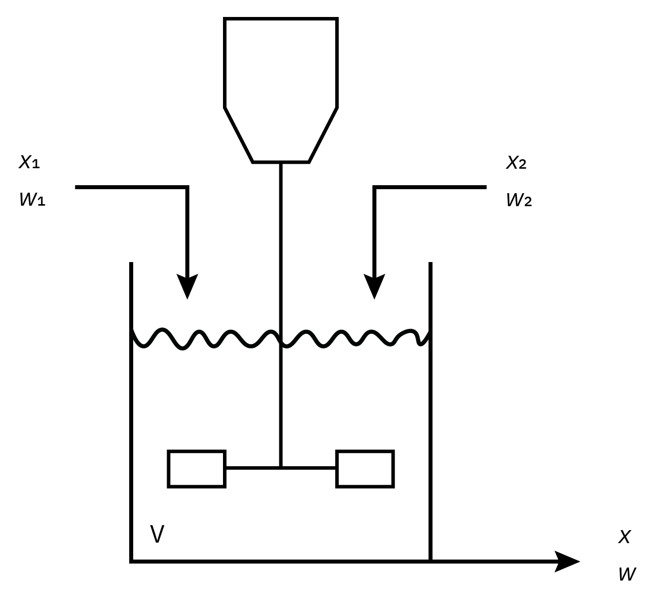
Overall mass balance
\left\{\begin{array}{c} \text {rate of accumulation} \\ \text {of mass in the tank} \end{array}\right\} = \left\{\begin{array}{c} \text {rate of} \\ \text {mass in} \end{array}\right\} - \left\{\begin{array}{c} \text {rate of} \\ \text {mass out} \end{array}\right\}
\frac{d(V \rho)}{dt} = w_1 + w_2 - w
Component balance
\frac{d(V \rho x)}{dt} = w_1 x_1 + w_2 x_2 - w x
Blending of two components
Overall mass balance
\left\{\begin{array}{c} \text {rate of accumulation} \\ \text {of mass in the tank} \end{array}\right\} = \left\{\begin{array}{c} \text {rate of} \\ \text {mass in} \end{array}\right\} - \left\{\begin{array}{c} \text {rate of} \\ \text {mass out} \end{array}\right\}
\frac{d(V \rho)}{dt} = w_1 + w_2 - w
Component balance
\frac{d(V \rho x)}{dt} = w_1 x_1 + w_2 x_2 - w x
It is possible to further simplify the system of two differential equations to
\frac{dV}{dt} = \frac{1}{\rho}\left(w_1 + w_2 - w \right)
\frac{dx}{dt} = \frac{w_1}{V \rho} \left(x_1 - x\right)+ \frac{w_2}{V \rho} \left(x_2 - x\right)
Solution of model equations
Nonlinear Chemical Processes: These result in complex ordinary differential equations when modeled.
Linear System Controls: These tools are well-established and provide valuable insights when processes operate near a specific point.
Laplace Transform: This simplifies creation of input-output models by converting differential equations to algebraic ones.
Transfer Function: An essential tool in control system design and analysis, representing linear control theory.
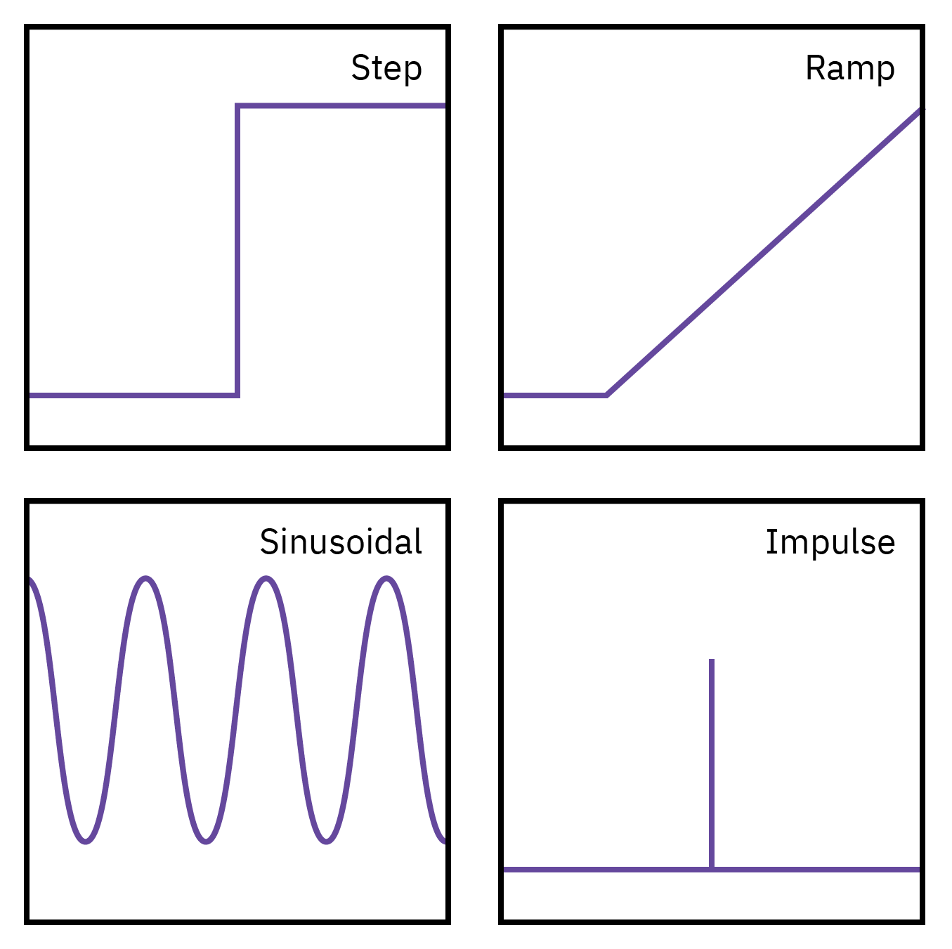
Input types
Response of first-order systems
Overall mass balance
A \frac{dh}{dt} = F_{in} - F_{out}
Outlet flow rate, Fout has a square-root dependence on liquid level F_{out} = \beta \sqrt{h}
Resulting nonlinear equation
A \frac{dh}{dt} = F_{in} - \beta \sqrt{h}
\tau \frac{d \bar{h}}{dt} + \bar{h} = kF_{in} ; \, \tau = \frac{2A\sqrt{h}}{\beta} ; \, k = \frac{2 \sqrt{h}}{\beta}
Transfer function
\frac{\bar{h}(s)}{\bar{F_in}(s)} = g(s) = \frac{k}{\tau s + 1}
Process gain (k): Ultimate value of the response (new steady-state) for a unit-step change in the input.
Time constant (τ): Time necessary for the process to adjust to a change in the input.
Response of first-order systems

The ultimate (steady-state) value of the response, \bar{h} (t \to \infty), is equal to k for a unit-step change.
When the elapsed time is equal to the process time constant t = \tau, the system reaches 63.2% of its final response.
After approximately 5τ, the transient response can be considered as having reached steady-state.
For a given t / τ, the output reaches the same fraction of the ultimate output response value.
In a tank process, a rise in the inlet flow rate elevates the liquid level, which in turn increases the hydrostatic pressure and subsequently the outlet flow rate. The system eventually reaches a new steady state. This feature is termed ‘self-regulation’.
Response of first-order systems

Response of second-order systems
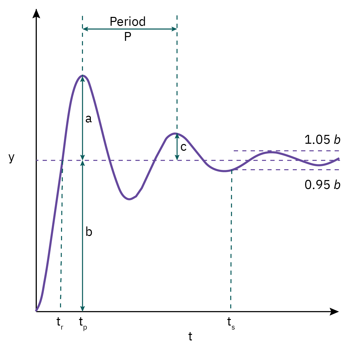
Rise time (t_r): time required for y(t) to first cross its new steady state value
Overshoot (a/b): The maximum amount by which the response exceeds the new steady state value
Decay ratio (c/a): Ratio of the height of successive peaks in the response
Period of oscillation (P): time for a complete cycle
Response/ settling time (t_s): time required for the response to remain within a ± 5% band based upon steady state value.
Decay ratio, overshoot, response time, and damping factor (ξ) can be used as a basis for tuning.
Response of second-order systems
Critically damped (ξ = 1)

Output response becomes more sluggish as τ increases.
The responses are qualitatively similar.
Effect of ξ

ξ < 1: Oscillation and overshoot
ξ > 1: Sluggish response, no oscillations; no overshoot
ξ = 1: Fastest response, no oscillations; no overshoot
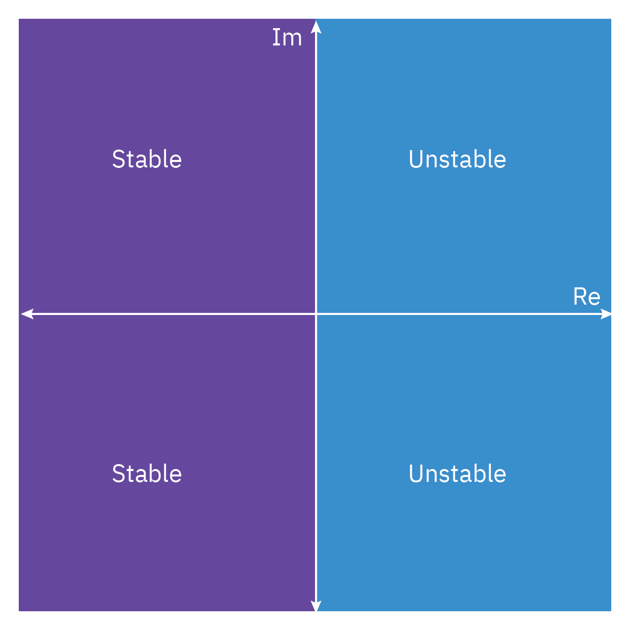
Stability of linear systems
- The location of the poles of a transfer function determines the bounded input–bounded output (BIBO) stability of a process.
- If the transfer function of a dynamic process has a pole with a positive real part, the process is unstable. If the real part is zero, then the process is critically stable
- We need to be cautious when we derive a transfer function model from a statespace model, because a zero (or zeros) may cancel a pole (or poles). This becomes especially important if the canceled pole is unstable, which means that those modes of the process would be hidden from us.
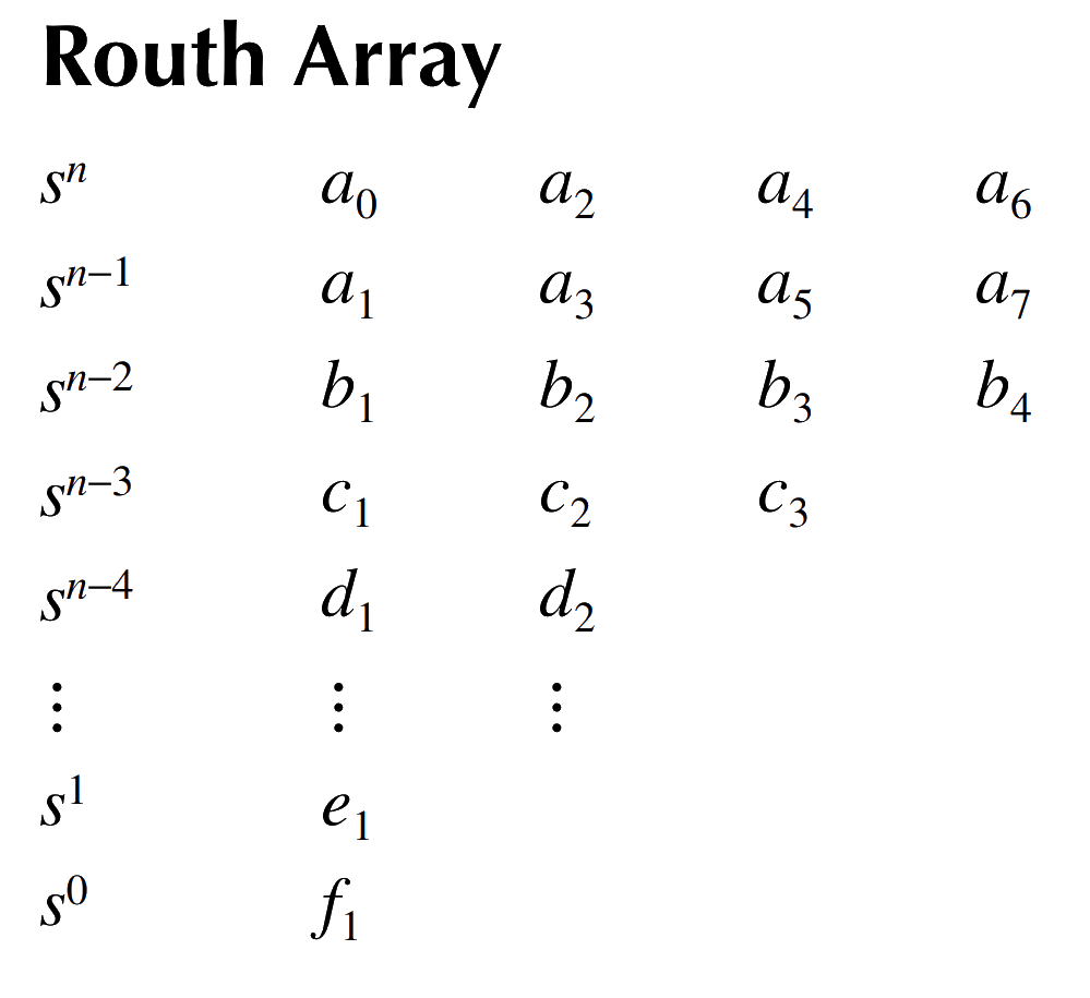
Routh’s Stability Criterion
Routh’s Criterion is a mathematical test that is used to determine whether a linear system is stable or unstable. It does not require explicit calculation of the roots of the characteristic equation.
Characteristic equation
a_0 s^n + a_1 s^{n-1} + a_2 s^{n-2} + \dots + a_n = 0
The first step in Routh’s Criterion is to set up the Routh array.
Then, we examine the first column of the array. If there are no sign changes in the first column, the system is stable.
If there are sign changes in the first column, the system is unstable. The number of sign changes corresponds to the number of roots with positive real parts.
Routh’s Criterion can also be used to determine relative stability and system type.
Root locus method
Root Locus is a graphical method used in control systems to examine how the system stability changes with varying gain.
It shows possible pole locations as system gain varies from zero to infinity.
The method provides insights into stability and transient response.
Root locus begins at open-loop poles and ends at open-loop zeros.
The plot exists on parts of the complex plane where the number of open-loop poles and zeros to the right is odd.
Consider the characteristic equation p(s,k)= s^2 + s + k =0

Introduction to feedback control

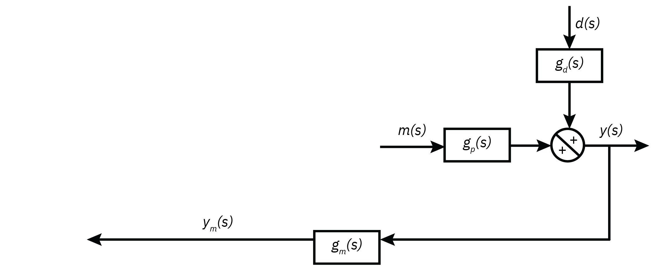
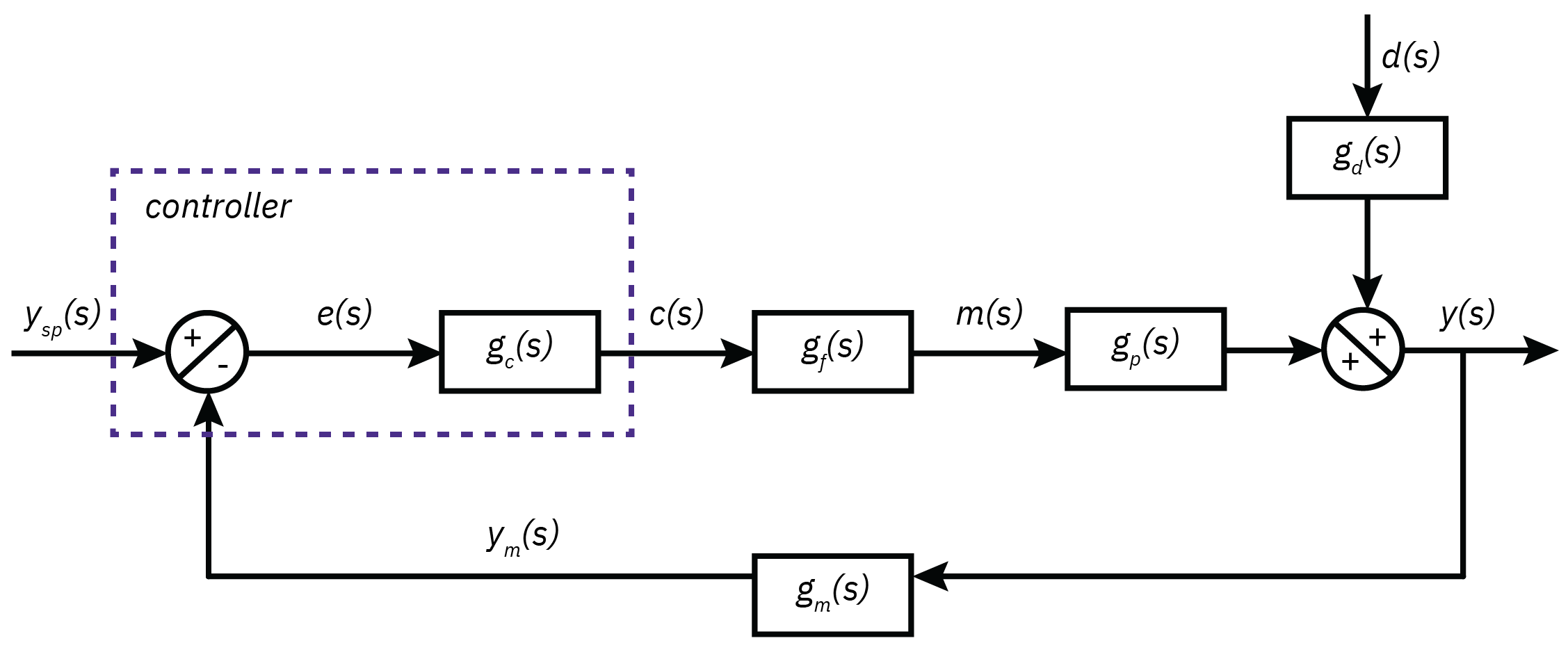
Introduction to feedback control
y = g_p m + g_d d
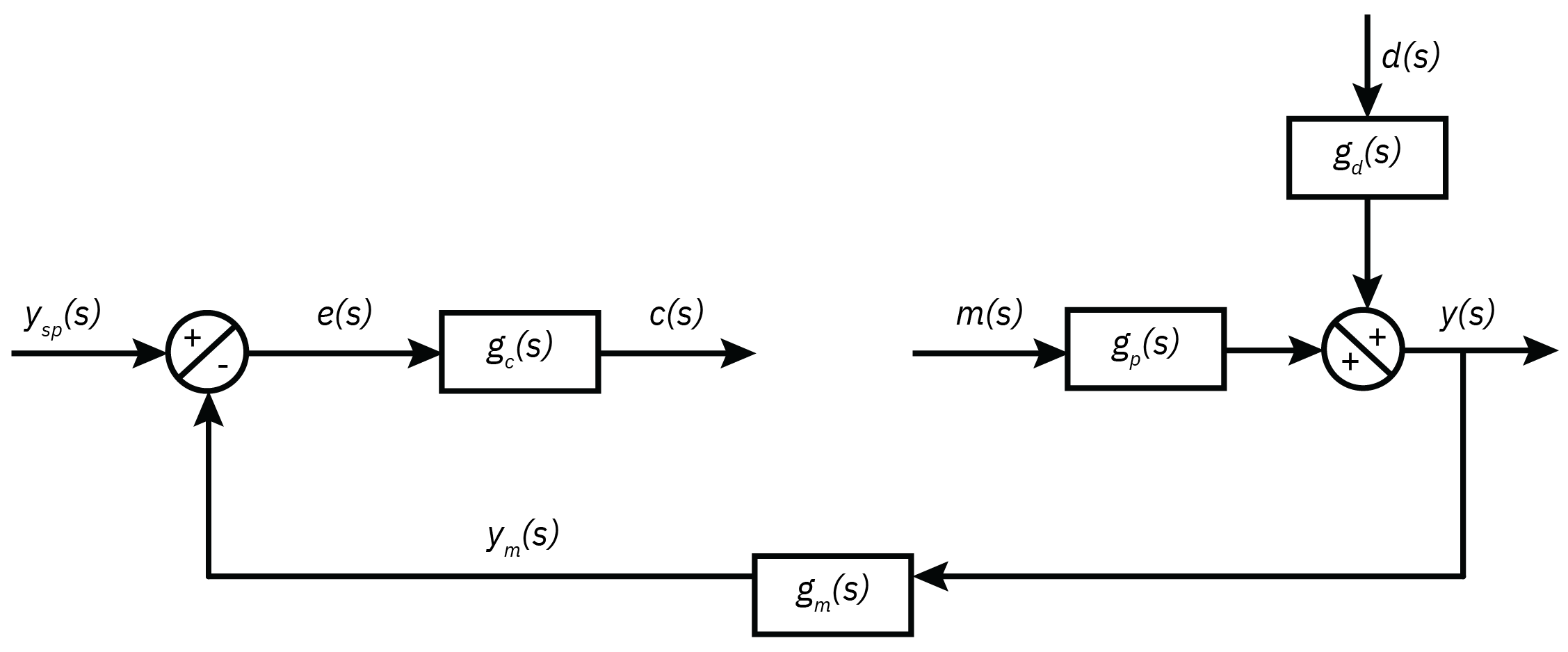
Error: e = y_{sp} - y_m
Control action: c = g_c e = g_c(y_{sp} - y_m)
Manipulated variable: m = g_f c = g_c g_f (y_{sp} - y_m)
Controlled variable: y = g_p m + g_d d = g_c g_f g_p (y_{sp} - y_m) + g_d d
Closed loop transfer function y = \frac{g_p g_f g_c}{1 + g_p g_f g_c g_m} y_{sp} + \frac{g_d}{1 + g_p g_f g_c g_m} d
Introduction to feedback control
Introduction to feedback control
Proportional mode

Integral mode

Derivative mode

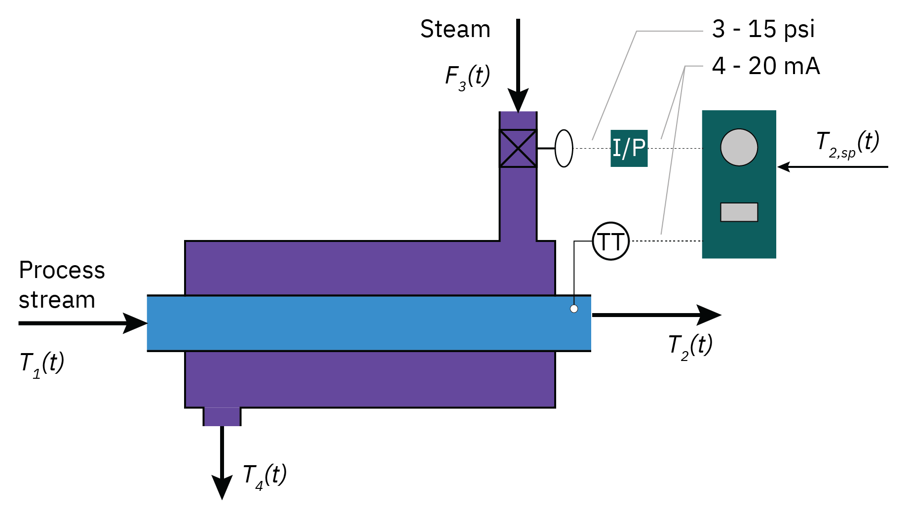
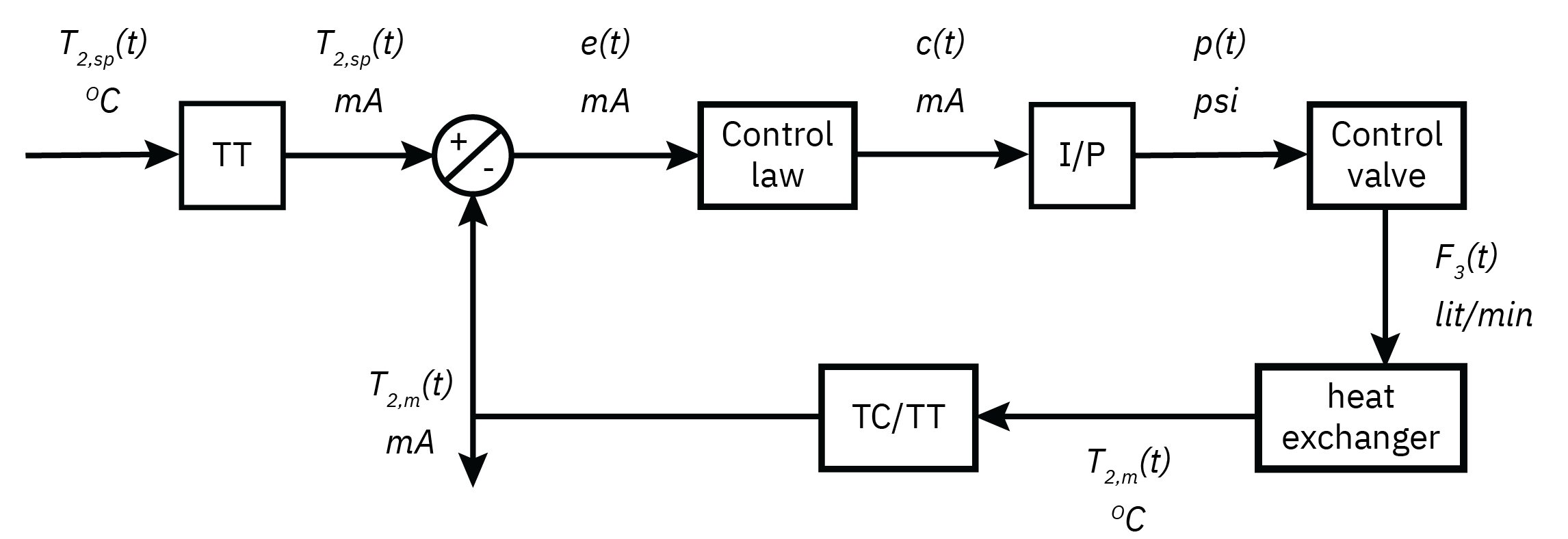
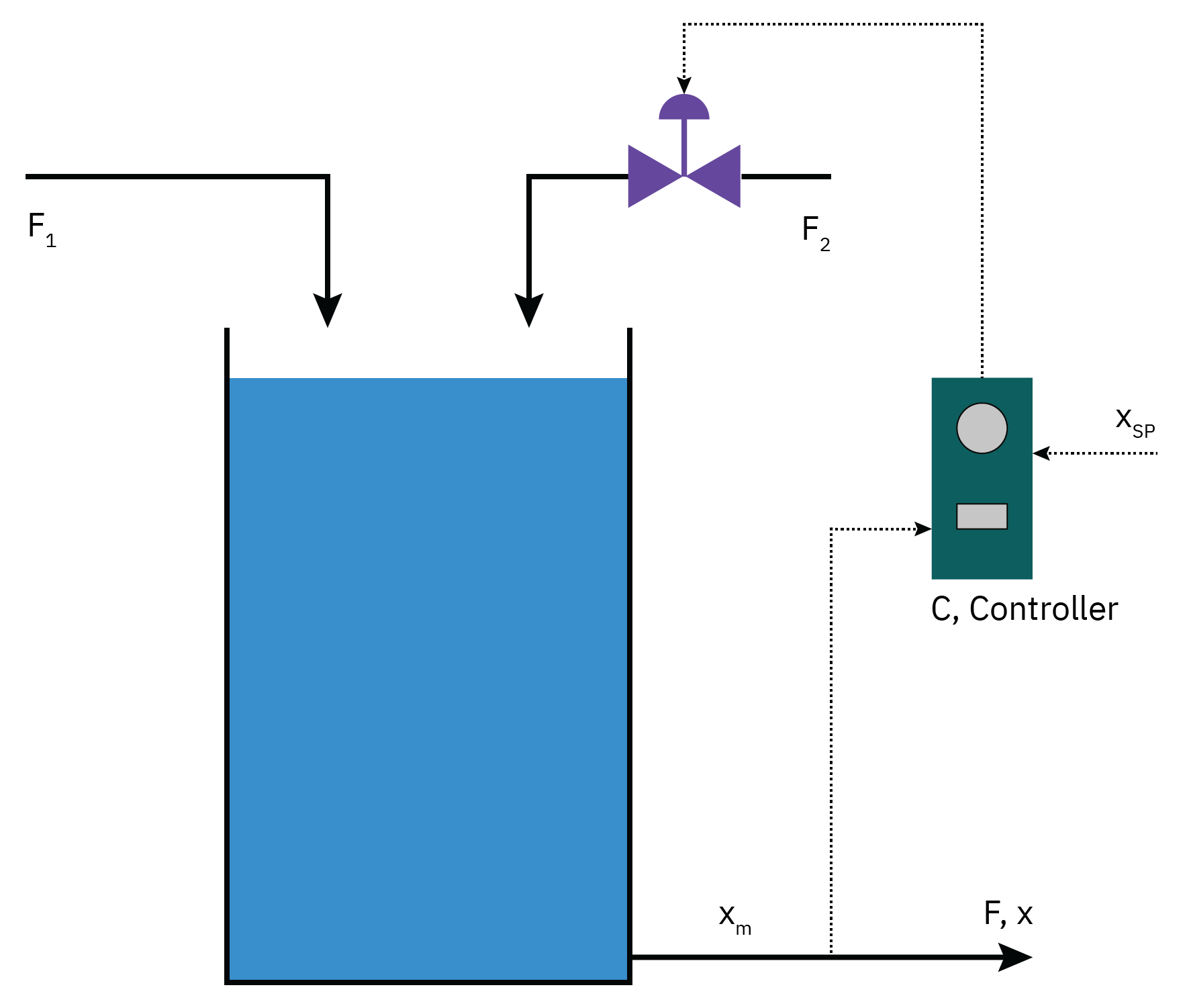
Mixing tank
The manipulated variable is the flow rate of stream 2, F_2, to control the outlet mass fraction, x.
The disturbance is the flow rate of stream 1, F_1.
The feed mass fractions are assumed constant.
There is a P controller, g_c(s) = k_c.
The dynamics of the actuators and the sensors are accounted for by pure dead-time elements, resulting in the transfer functions
\bar{x}(s) = \frac{-0.1 e^{-s}}{2.5s + 1} \bar{F}_1(s) + \frac{ 0.1 e^{-s}}{2.5s + 1} \bar{F}_2(s)
Mixing tank: setpoint change

Mixing tank: disturbance rejection
